Risk: an introduction

Risk of an event = Probability of the event happening × the consequensces of the event happening.¹

To understand probability better, please read this and this.

This is the most basic definition of Risk. Risk = Probability, or how likely an event is to occur × Consequence, or impact. Because it is multiplicative, a high-probability event with low consequence (losing a pen) is low risk, and a low-probability event with catastrophic consequence (say, a nuclear exchange) can be high risk. The danger zone is where meaningful probability meets serious consequence.

History
For most of history, people spoke about fate, luck, or divine will, not “risk” in a calculable sense. Hazards (storms, plagues, crop failures) were seen as acts of gods or nature. There was no notion of systematically measuring uncertainty.

In the 17th Century, A French nobleman, Chevalier de Méré, asked Blaise Pascal why some gambling bets worked better than others. Pascal’s correspondence with Pierre de Fermat (1654) is widely seen as the birth of modern probability theory.²³ They developed early ideas of expected value – essentially, the mathematical ancestor of “probability × impact”.⁴

In the 18th Century, Daniel Bernoulli introduced the idea of utility in 1738:⁵ the insight that losing or gaining the same amount (£100) does not feel equally important to rich and poor people. This work planted the seeds for understanding why humans are risk‑averse and set the stage for later behavioural theories.

As trade, shipping and life insurance developed in the 18th–19th centuries, people started using probability tables to price the risk of death, shipwrecks and fire.⁶ This was the first large‑scale, institutional attempt to put numbers on everyday risks and pool them.⁶ Risk pooling is when lots of people chip in a little money into a shared pot (the “pool”) so that when one person has a big, unexpected cost (like a car accident or sickness), the money from the whole group covers it, making big losses manageable for individuals and premiums more stable for everyone.⁷ After industrialisation, wars and technological disasters, “risk” broadened from individual hazards (a ship sinking) to complex systems (nuclear power, financial markets, supply chains). The language of “risk management” emerged after the Second World War and matured through the later 20th century, culminating in general standards such as ISO 31000.⁸⁹

Expected Value⁹¹⁰
The mathematical heart of risk is Expected Value (EV). This is simply the average outcome if you repeated an action infinitely.

If a bet offers a 50% chance to win £100 and a 50% chance to lose nothing, the Expected Value is £50 ($0.50 \times 100 + 0.50 \times 0$). Rationally, you should pay anything up to £49.99 to take that bet.

But real life isn’t a casino with infinite replays. Humans often get only one shot. If an individual takes a risk with a positive expected value—like cycling to work to save money and improve health—but gets hit by a bus on day one, the “average” outcome is irrelevant. This is why variance matters as much as the average. A risk might look good on paper (high expected value) but have a “ruin condition” (a consequence you can’t recover from) that makes the math irrelevant.

Normal Distribution
If you measured the height of every single individual on the planet, or even a representative sample of them, the shape of that graph (often called “curve” in academic language) would be similar to this image:

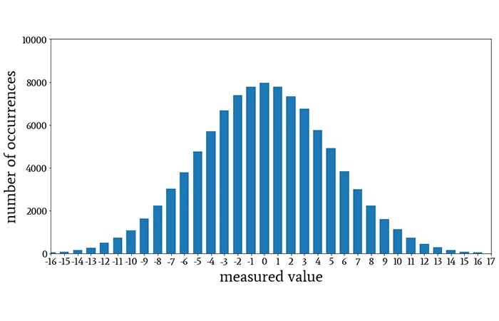
This is the Normal Distribution (or Bell Curve), and it is the most important shape in risk management.¹² It describes how randomness usually behaves. The very top of the hill represents the Mean (the average). This is what you “expect” to happen; in our stadium example, this is the average height (say, 5’9″). The vast majority of people will be average height, so their heights will be recorded as being clustered right around the middle.

If the Mean tells you where the peak is, Variance tells you how wide the hill is. It is a statistical measure showing how spread out a set of data points are from their average.¹³

• Low Variance: Imagine a hill that looks like a needle. This means data points are tightly clustered. If you measured the height of 10,000 professional jockeys, the variance would be low—almost everyone is close to the average.¹⁴
• High Variance: Imagine a hill that looks like a flattened pancake. This means data is widely spread out. If you measured the height of a random crowd containing jockeys and basketball players, the hill would be very wide.¹⁵

In risk management, mean tells you what usually happens; variance measures unpredictability and the potential for outcomes to be very different from the average, which is the essence of uncertainty.¹⁶¹⁷ A high variance means numbers are widely scattered, increasing the chance of both extreme positive and, crucially, extreme negative outcomes (losses).¹⁸ Low variance indicates they are clustered closely around the mean: it quantifies the dispersion or variability within a dataset.¹⁸ In the height data set, while most people would be average height, some people would be very short and others very tall as well. It’s just that the number of people who are not close to the average would fall off the farther away we get from the mean, or the middle of the bell curve.

Standard Deviation¹⁸¹⁹

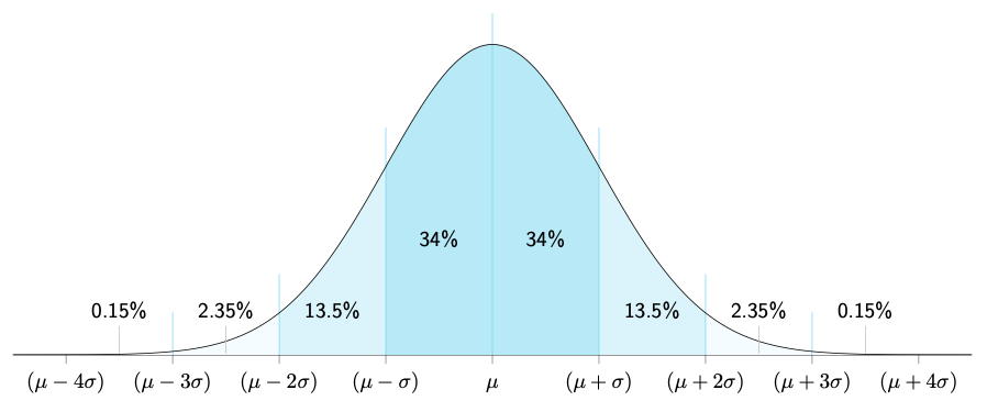
If Variance tells you the hill is “wide,” Standard Deviation (Sigma, or σ) tells you exactly how wide in real units. It is simply the square root of variance.

Think of Standard Deviation as the ruler for the Bell Curve.

• 1 Standard Deviation: In a normal distribution, about 68% of all outcomes happen within one standard deviation of the mean. If the average height is 5’9″ and the standard deviation is 3 inches, 68% of men are between 5’6″ and 6’0″.
• 2 Standard Deviations: Go out a bit further, and you capture 95% of all outcomes.
• 3 Standard Deviations: Go out three steps, and you capture 99.7% of everything.

In risk, when someone talks about a “Six Sigma” event (six standard deviations away from the average), they are talking about something so rare that it should theoretically almost never happen. And yet, in financial markets and complex systems, these “impossible” events happen surprisingly often.

Confidence²¹²²
If a bank says, “We are 95% confident we won’t lose more than £1 million tomorrow,” they are essentially saying: “If tomorrow is a normal day (one of the 95%), we are safe. But if tomorrow is one of those rare, 1-in-20 bad days, all bets are off.”

In statistics, confidence is often explained using confidence intervals: at a 95% confidence level, the method used to build the interval would capture the true value about 95 times out of 100 repeated samples. That does not mean the true value has a 95% probability of being inside this specific interval; it means the procedure has 95% long-run reliability. This means, confidence intervals speak about frequency: how often do the unexpected or unwanted events happen. At 95%, they happen on any 5 days out of 100. at 99%, they happen once every 100 days.

For risk management, think of confidence levels as a dial for paranoia:

• 95% Confidence: You are planning for the normal bad days. You accept that on 1 day out of every 20 (roughly once a month), you will breach your limit.
• 99% Confidence: You are planning for the severe days. You only accept breaching your limit on 1 day out of 100 (roughly 2–3 times a year).
• 99.9% Confidence: You are planning for near-disaster. You only accept a breach once every 1,000 days (roughly once every 4 years).

The Micromort
In the 1970s, Stanford professor Ronald Howard needed a way to compare diverse risks like skydiving, smoking, and driving. He invented the Micromort—a unit representing a one-in-a-million chance of death.²³

This equalises different activities. Instead of vague fears (“is it safe to fly?”), we can use units:

• 1 Micromort is roughly the risk of driving 250 miles (400 km).²⁴
• 1 Micromort is also the risk of flying 6,000 miles (9,600 km).²⁴
• Scuba diving costs about 5 micromorts per dive.²⁵
• Skydiving costs about 8–10 micromorts per jump.²⁴
• Just being alive (all-cause mortality for a young person) costs roughly 1 micromort per day.²⁶

In conclusion, risk is the price of life.

Sources

1. ISO 31000 Risk Management Process – Practical Risk Training
2. July 1654: Pascal’s Letters to Fermat on the “Problem of Points” – APS News
3. How a Letter Between Two Mathematicians in 1654 Changed the Way We View the Future – KPBS
4. Pascal and Fermat (1654) – Ebrary
5. Daniel Bernoulli (1738): Evolution and Economics Under Risk – UBC Zoology (PDF)
6. The History of Insurance: From Ancient Risk to Modern Protection – Briggs Agency
7. Risk Pooling: How Health Insurance Works – American Academy of Actuaries
8. The Evolution of Risk Management: Lessons from History – Risk Management Strategies
9. Expected Value Calculator – Omnicalculator
10. Expected Value in Statistics: Definition and Calculation – Statistics How To
11. Introduction to Gaussian Distribution – All About Circuits
12. Empirical Rule (68-95-99.7) Explained – Built In
13. Calculate Standard Deviation & Variance – SurveyKing
14. What is considered a high or low variance? – Reddit r/mathematics
15. Variance in Statistics – GeeksforGeeks
16. Risk-Managing the Uncertainty in VaR Model Parameters – Research Affiliates (PDF)
17. The Risks of Uncertainty – ACCA Global
18. Variance – GeeksforGeeks
19. Empirical Rule: Definition & Formula – Statistics by Jim
20. Normal Distribution Diagram – TikZ.net
21. Definition: Confidence Level – Statista
22. The Role of Confidence Levels in Statistical Analysis – Statsig
23. There’s a Small Chance This Article May Kill You (Micromorts) – Portable Press
24. Quantifying Risk – GS Trust Co
25. Understanding DAN’s Accident Data – Alert Diver Magazine
26. Microlives: A Lesson in Risk Taking – BBC Future