Climate Change – Page 2

GHG Accounting: ISO 14064-1

Note: I know this is quite technical, but it’s about accounting, so that’s natural. Financial accounting tends to be technical too, right?

The ISO 14064 series is a family of international standards by the International Organization for Standardization (ISO) for quantification, monitoring, reporting, and verification of GHG emissions. They were developed by Technical Committee ISO/TC 207 on Environmental Management, Subcommittee SC 7 on Greenhouse Gas Management, can be adopted across different sectors, regions, and organisational types.

The ISO 14064 series currently comprises four main parts:

ISO 14064-1:2018 – “Greenhouse gases – Part 1: Specification with guidance at the organisation level for quantification and reporting of greenhouse gas emissions and removals.” This standard enables organisations to measure and report their total greenhouse gas emissions and removals.
ISO 14064-2:2019 – “Greenhouse gases – Part 2: Specification with guidance at the project level for quantification, monitoring and reporting of greenhouse gas emission reductions or removal enhancements.” This standard applies to specific projects designed to reduce emissions or enhance carbon removals, such as renewable energy installations, energy efficiency retrofits, reforestation programs, or methane capture projects.
ISO 14064-3:2019 – “Greenhouse gases – Part 3: Specification with guidance for the verification and validation of greenhouse gas statements.” This standard provides the framework for independent third-party verification and validation of GHG claims. It is the assurance mechanism that gives stakeholders confidence in reported emissions data.
ISO/TS 14064-4:2025 – “Greenhouse gases – Part 4: Guidance for the application of ISO 14064-1.” This newest addition, published in November 2025, is a Technical Specification that provides practical, step-by-step guidance for implementing ISO 14064-1. It bridges the gap between the normative requirements of the standard and real-world application, with detailed examples and case studies for different organisational types and sectors.

Additionally, the broader ISO 14060 family includes ISO 14065:2020 (requirements for bodies validating and verifying GHG statements), ISO 14066:2023 (competence requirements for verifiers and validators), and ISO 14067:2018 (carbon footprint of products).

This ecosystem of standards creates a framework:

Organisations use ISO 14064-1 and 14064-4 to calculate their emissions;
Project developers use ISO 14064-2 to quantify project benefits;
Independent verifiers use ISO 14064-3 to audit these claims; and a
Accreditation bodies use ISO 14065 and 14066 to ensure the competence and impartiality of the verifiers themselves.

The Five Core Principles

Relevance: Select the GHG sources, GHG sinks, GHG reservoirs, data and methodologies appropriate to the needs of the intended user.
Completeness: Include all relevant GHG emissions and removals.
Consistency: Enable meaningful comparisons in GHG-related information.
Accuracy: Reduce bias and uncertainties as far as is practical.
Transparency: Disclose sufficient and appropriate GHG-related information to allow intended users to make decisions with reasonable confidence.

As stated explicitly in ISO 14064-1, “The application of principles is fundamental to ensure that GHG-related information is a true and fair account. The principles are the basis for, and will guide the application of, the requirements in this document”.

Relevance: Appropriateness to User Needs
This principle recognises that GHG inventories and reports serve specific purposes and must be designed to meet the needs of those who will rely on the information to make decisions.

Relevance begins with clearly identifying the intended users of the GHG inventory and understanding their information needs. Intended users may include the organisation’s own management, investors, lenders, customers, regulators, GHG programme administrators, or other stakeholders. Different users may have different information needs. For example, investors may focus primarily on climate-related financial risks and opportunities, while regulators may require specific emissions data for compliance purposes.

The relevance principle requires organisations to make appropriate boundary decisions (determining which operations, facilities, and emissions sources to include in the inventory based on what is material and meaningful to intended users): an inventory that excludes significant emission sources or includes irrelevant information fails to serve user needs effectively.

In practice, applying the relevance principle means that organisations must engage with their stakeholders to understand what information they need and why, design inventory boundaries and methodologies to provide this information, focus effort on quantifying the most significant emissions sources, and regularly reassess whether the inventory continues to meet user needs as circumstances change.

Completeness: Including All Relevant Emissions
The completeness principle requires organisations to include all relevant GHG emissions and removals within the chosen inventory boundaries. This principle ensures that GHG inventories provide a comprehensive picture of an organisation’s climate impact rather than selectively reporting only favorable information.

Completeness operates at multiple levels. At the broadest level, it requires that organisations establish appropriate organisational and reporting boundaries and then include all sources and sinks within those boundaries. For organisational-level inventories under ISO 14064-1, this means accounting for all facilities and operations that fall within the defined organisational boundary, whether based on control or equity share. It also means including both direct emissions from sources owned or controlled by the organisation and indirect emissions that are consequences of organisational activities.

The 2018 revision fundamentally changed how organizations handle indirect emissions. Instead of treating “Scope 3” as a monolithic category, ISO now requires systematic evaluation across six specific categories. This shift reflects reality: a manufacturer’s supply chain emissions (Category 4) and product use-phase emissions (Category 5) are fundamentally different and require different strategies. Organisations must systematically identify potential sources of indirect emissions throughout their value chains and include those that are determined to be significant based on magnitude, influence, risk, and stakeholder concerns. The real problem here is data availability: an organisation might know its own production emissions precisely, but will struggle to get Scope 3 data from thousands of distributors, and this makes implementation messy and imprecise.

An important aspect of completeness is the treatment of exclusions. If specific emissions sources or greenhouse gases are excluded from the inventory, ISO 14064-1 requires organisations to disclose and justify these exclusions. Justifications must be based on legitimate reasons such as immateriality, lack of influence, or technical measurement challenges, not simply on a desire to report lower emissions.

For GHG projects under ISO 14064-2, completeness requires identifying and quantifying emissions and removals from all relevant sources, sinks, and reservoirs affected by the project, including controlled, related, and affected SSRs. Failure to account for emission increases from affected sources (often called leakage) would result in overstatement of project benefits.

Consistency: Enabling Meaningful Comparisons
The consistency principle requires that organisations enable meaningful comparisons in GHG-related information over time and, where relevant, across organisations. Consistency is essential for tracking progress toward emission reduction targets, assessing the effectiveness of mitigation initiatives, and enabling external stakeholders to compare performance across organisations or sectors.

Consistency has several dimensions. It requires using consistent methodologies, boundaries, and assumptions over time when quantifying and reporting emissions. When an organisation measures its emissions in one year using specific methodologies and emission factors, it should apply the same approaches in subsequent years to enable valid comparisons.

It is important to note that consistency does not mean organisations can never improve their methodologies or expand their boundaries. Organisations may and should refine their approaches over time to improve accuracy, expand scope, or respond to changing circumstances. However, when such changes occur, consistency requires transparent documentation of what changed and why, recalculation of prior years where necessary to maintain comparability, and clear explanation in reports so users understand the nature and impact of changes.

Case in point, the base year concept embodied in ISO 14064-1 is central to applying the consistency principle. Organisations select a specific historical period as their base year against which future emissions are compared. The base year serves as the reference point for measuring progress toward reduction targets. ISO 14064-1 requires organisations to establish policies for recalculating base year emissions when significant changes occur to organisational structure, boundaries, methodologies, or discovered errors. These recalculation policies ensure that year-over-year comparisons remain valid even as organisations evolve.

The recalculation policy is most commonly triggered by three types of organisational change. First, structural changes: acquisitions, divestitures, or mergers that materially alter the scope of operations. ISO 14064-1 and the GHG Protocol typically define “material” as changes exceeding 5% of Scope 1 and Scope 2 emissions in the base year. For example, if a retail company acquires a logistics provider representing an additional 6% of historical emissions, the base year must be recalculated to include that logistics provider, enabling fair year-on-year comparison. Second, methodology improvements: when an organisation discovers better data or more appropriate emission factors. If a facility previously used regional electricity emission factors but gains access to grid-specific data, or if a company previously estimated employee commuting emissions using averages but now collects actual commute data, these improvements warrant recalculation. The driver is not change for its own sake, but the principle that prior years should benefit from improved accuracy just as current years do. Third, discovered errors: when an organisation identifies that prior-year calculations were systematically wrong—either over or understating emissions—recalculation is not optional; it is mandatory. Transparency requires disclosing both the error and its magnitude, then correcting the historical record. Organisations often establish a threshold (commonly 5%) below which minor corrections do not trigger full recalculation; instead, they are noted as adjustments in the current year.

Accuracy: Reducing Bias and Uncertainty
Accuracy involves reducing systematic bias and reducing uncertainty.

Systematic bias occurs when quantification methods consistently overstate or understate actual emissions. For example, using an emission factor that is inappropriately high or low for the specific activity being quantified would introduce bias. The accuracy principle requires ensuring that quantification approaches are systematically neither over nor under actual emissions, as far as can be judged.
Uncertainty refers to the range of possible values that could be reasonably attributed to a quantified amount. All emission estimates involve some degree of uncertainty arising from measurement imprecision, estimation methods, sampling approaches, lack of complete data, or natural variability. The accuracy principle requires reducing these uncertainties as far as is practical through using high-quality data, appropriate methodologies, and robust measurement and calculation procedures. ISO 14064-1 requires organisations to assess uncertainty in their GHG inventories, providing both quantitative estimates of the likely range of values and qualitative descriptions of the causes of uncertainty. This assessment helps organisations identify where improvements in data quality or methodology could most effectively reduce overall inventory uncertainty.

Achieving accuracy begins with selecting appropriate quantification approaches. ISO 14064-1 recognises multiple approaches to quantification, including direct measurement of emissions, mass balance calculations, and activity-based calculations using emission factors. The most accurate approach depends on the specific source, data availability, and the significance of the emission source.

Organisations should also prioritise primary data (data obtained from direct measurement or calculation based on direct measurements) over secondary data from generic databases. Site-specific data obtained within the organisational boundary is preferable to industry-average or regional data. However, the accuracy principle also recognises practical constraints—perfect accuracy is often unachievable and unnecessary, particularly for minor emission sources.

The requirement to separately report biogenic CO₂ from fossil fuel CO₂ in Category 1 may seem like a technical distinction, but it reflects a fundamental policy divergence emerging globally. Biogenic emissions arise from the combustion of biomass (wood, agricultural waste, biogas) and are considered part of the natural carbon cycle—the carbon released was recently absorbed by growing plants or waste decomposition. Fossil emissions, by contrast, release carbon that has been sequestered for millions of years. Regulatory frameworks increasingly treat these differently. The European Union’s Emissions Trading System (EU ETS) has updated its carbon accounting rules multiple times to refine biogenic CO₂ treatment; the GHG Protocol has issued separate guidance; and emerging carbon credit schemes apply different rules depending on biogenic versus fossil origin. An organisation that reports these separately today is insulated from tomorrow’s regulatory changes. If a company bundles biogenic and fossil emissions together, it cannot easily disaggregate them later without recalculating historical data. Practically, this means a biomass energy facility, a wastewater treatment plant using anaerobic digestion, or a manufacturer using wood waste for process heat must track biogenic emissions in their systems from the outset.

Transparency: Disclosing Sufficient Information
The transparency principle requires that organisations disclose sufficient and appropriate GHG-related information to allow intended users to make decisions with reasonable confidence. Transparency is fundamental to building trust and credibility in GHG reporting—it enables users to understand what was measured, how it was measured, and what limitations exist in the reported information.

Transparency requires that organisations address all relevant issues in a factual and coherent manner, based on a clear audit trail. This means documenting the assumptions, methodologies, data sources, and calculations used to quantify emissions such that an independent party could understand and reproduce the results.

The transparency principle requires that a reader—whether a regulator, investor, or internal stakeholder—could theoretically follow the same calculation path and reach the same answer. This demands more than good intentions; it requires structural discipline in documentation. In practice, an effective audit trail captures the decision journey, not just the numbers. It documents: which emissions sources were identified as material (and why), which were excluded (and why), what data was collected and from which sources, which assumptions were necessary (e.g., assumed product lifespans, allocation methods for shared facilities), what methodologies were applied, and crucially, where uncertainty remains. For example, a beverage manufacturer’s Scope 3 inventory might document that it obtained actual emissions data from 60% of direct suppliers (by volume) but relied on industry-average factors for the remaining 40%. That gap is not hidden; it is documented as a source of uncertainty in the overall inventory. This approach serves two audiences simultaneously. Internal management gains confidence that the number is defensible. External verifiers and stakeholders understand the methodology’s strengths and limitations, enabling better-informed decisions.

A clear audit trail is essential to transparency. Organisations should maintain robust documentation that traces emissions from source data through calculations to final reported totals. This documentation should include:

descriptions of organisational and reporting boundaries;
lists of emission sources and sinks included in the inventory;
methodologies and emission factors used for each source category;
activity data, sources of data, and data collection procedures;
calculations and any assumptions made; and
any exclusions and the justifications for excluding specific sources.

Transparency requires disclosing not only the final emission totals but also the information needed to understand and evaluate those totals. ISO 14064-1 specifies extensive requirements for what must be included in GHG reports, including both mandatory and recommended disclosures. These disclosures cover methodological choices, data quality, uncertainty, significant changes from previous years, verification status, and other information relevant to interpreting the reported emissions.

The transparency principle also requires acknowledging limitations and uncertainties in the reported information. Rather than implying false precision, organisations should clearly communicate where significant uncertainties exist, what assumptions were necessary, and what information was unavailable or excluded. This honest acknowledgment of limitations enhances rather than diminishes credibility, as it demonstrates rigorous and objective assessment.

Establishing Organisational Boundaries
The first step in developing a GHG inventory is determining organisational boundaries, which means that the organisation should define what operations, facilities, and entities are included in the inventory based on the organisation’s relationship to them.

ISO 14064-1 allows organisations to choose from two primary consolidation approaches:

Equity share approach: The organisation accounts for its proportional share of GHG emissions and removals from facilities based on its ownership percentage. The equity share reflects economic interest, which is the extent of rights a company has to the risks and rewards flowing from an operation. Typically, the share of economic risks and rewards in an operation is aligned with the company’s percentage ownership of that operation, and equity share will normally be the same as the ownership percentage. Where this is not the case, the economic substance of the relationship the company has with the operation always overrides the legal ownership form to ensure that equity share reflects the percentage of economic interest.
Control approach (financial or operational): The organisation accounts for 100% of GHG emissions and removals from facilities over which it has financial or operational control, and 0% from facilities it does not control.
- Under the operational control approach, an organisation has operational control over a facility if the organisation or one of its subsidiaries has the authority to introduce and implement its operating policies at the facility. This is the most common approach, as it typically aligns best with what an organisation feels it is responsible for and often leads to the most comprehensive inclusion of assets in the inventory.
- Under the financial control approach, an organisation has financial control over a facility if the organisation has the ability to direct the financial and operating policies of the facility with a view to gaining economic benefits from its activities. Industries with complex ownership structures may be more likely to follow the equity share approach to align the reporting boundary with stakeholder interests.

The choice of consolidation approach should be consistent with the intended use of the inventory and ideally align with how the organisation consolidates financial information. For example, an organisation that consolidates its financial statements based on operational control should typically use operational control for GHG inventory boundaries as well.

Boundary Consistency with Financial Reporting: Why It Matters
The ISO standard recommends (and increasingly, regulators require) that the consolidation approach used for GHG accounting align with the approach used for financial reporting. This is more than administrative convenience. When a company consolidates financial statements using operational control, its financial stakeholders are accustomed to seeing 100% of controlled operations reflected in results. If the GHG inventory uses a different boundary—say, equity share for a joint venture while the finance team uses operational control—the GHG data will seem inconsistent and raise credibility questions. More importantly, alignment simplifies assurance. An auditor examining both financial and GHG statements does not have to reconcile conflicting boundary interpretations. A company that uses control for finance but equity share for emissions is signalling (intentionally or not) that its GHG report is using a narrower or broader lens than its financial results, inviting scrutiny about whether the difference is justified or opportunistic. Alignment also supports integrated reporting. Increasingly, investors want to see how GHG emissions correlate with financial performance—emissions intensity (tonnes CO₂e per unit of revenue, per unit of asset, per FTE), carbon risk premium, or abatement costs. These correlations only make sense if the boundary is consistent.

Defining Reporting Boundaries: The Six-Category Structure
Once organisational boundaries are established, organisations must define their reporting boundaries—what types of emissions and removals are quantified and reported within the organisational boundary.

The 2018 revision of ISO 14064-1 introduced a significant innovation: a six-category structure for classifying emissions and removals. This structure evolved from and builds upon the GHG Protocol’s three-scope approach (Scope 1 for direct emissions, Scope 2 for energy indirect emissions, Scope 3 for all other indirect emissions). The ISO categories provide more granular classification of indirect emissions, facilitating identification and management of specific emission sources throughout the value chain.

Category 1: Direct GHG emissions and removals: Direct GHG emissions are emissions from GHG sources owned or controlled by the organisation. These are emissions that occur from operations under the organisation’s direct control—for example, emissions from combustion of fuels in company-owned vehicles or boilers, emissions from industrial processes at company facilities, or fugitive emissions from refrigeration equipment owned by the company. Organisations must quantify direct GHG emissions separately for CO₂, CH₄, N₂O, NF₃, SF₆, and other fluorinated gases. Additionally, ISO 14064-1 requires organisations to report biogenic CO₂ emissions separately from fossil fuel CO₂ emissions in Category 1. This separate reporting recognises that biogenic emissions may have different policy treatments, impacts, and implications than fossil emissions.

Category 2: Indirect GHG emissions from imported energy: This category includes indirect emissions from the generation of imported electricity, steam, heat, or cooling consumed by the organisation. When an organisation purchases electricity, the emissions from generating that electricity occur at the power plant (not owned by the organisation), but they are a consequence of the organisation’s decision to purchase and consume electricity. ISO 14064-1 requires organisations to report all Category 2 emissions, making this a mandatory category alongside Category 1.

Category 3: Indirect GHG emissions from transportation: This category includes emissions from transportation services used by the organisation but operated by third parties. Examples include emissions from business travel on commercial airlines, shipping of products by third-party logistics providers, and employee commuting.

Category 4: Indirect GHG emissions from products used by the organisation: This category includes emissions that occur during the production, transportation, and disposal of goods purchased by the organisation. Examples include emissions from the manufacturing of products the organisation buys, emissions from transporting materials used to make those products, and emissions from disposing of waste created by using those products. The boundary for Category 4 is “cradle-to-gate” from the supplier’s perspective—all emissions associated with producing and delivering products to the organisation.

Category 5: Indirect GHG emissions associated with the use of products from the organisation: This category includes emissions generated by the use and end-of-life treatment of the organisation’s products after their sale. When certain data on products’ final destination is not available, organisations develop plausible scenarios for each product. This category is particularly significant for manufacturers, as use-phase emissions from products often exceed emissions from manufacturing. For example, the emissions from operating a vehicle over its lifetime typically far exceed the emissions from manufacturing it.

For many product-based companies, Category 5 is the elephant in the room. An automotive manufacturer might account for 15–20% of its footprint in manufacturing emissions (Category 1) and another 10% in supply chain emissions (Category 4), but 50%+ in the use phase (Category 5). A household appliance manufacturer faces a similar dynamic—the electricity consumed by an appliance over its 15-year lifespan vastly exceeds the emissions from manufacturing. This creates strategic tension. The organisation has direct control over manufacturing efficiency—it can redesign processes, source renewable energy, or substitute materials. But use-phase emissions depend on the consumer’s electricity grid (which it does not control) and user behaviour (how often and how long the appliance runs). Yet ISO 14064-1 requires organisations to quantify these use-phase emissions and report them transparently, because stakeholders—particularly investors and policymakers—need to understand the full climate footprint of the products being sold. When data on product final destination is unavailable (e.g., a smartphone manufacturer doesn’t know where each unit is sold, or how long consumers keep it), ISO 14064-1 allows organisations to develop “plausible scenarios”—reasonable assumptions about usage patterns, product lifetime, and grid composition. These scenarios must be documented and justified, and they should be reassessed as more data becomes available or as circumstances change (e.g., grid decarbonisation).

Category 6: Indirect GHG emissions from other sources: This category captures any indirect emissions that do not fall into Categories 2-5. It serves as a catch-all to ensure completeness while avoiding double-counting. Organisations must be careful not to count the same emissions in multiple categories—for example, if emissions from a vehicle are included in Category 3 (transportation), they should not also be included in Category 4 (products) if the vehicle was used to transport a product.

Quantifying Emissions: Global Warming Potential and CO₂ Equivalent

GHG 101 – II: The Scope 3 Problem

A note before we begin: All scientific numbers here are estimates based on assessments available as of early 2025. They rely on complex climate modelling and come with uncertainty ranges.

Carbon accounting provides organisations with a systematic framework to measure, track, and report their greenhouse gas emissions. This helps both the organisation and external stakeholders understand environmental impact, set reduction targets, track progress, and make informed decisions about where to focus climate efforts.1

Carbon accounting isn’t just an academic exercise—it’s become essential for several interconnected reasons:2

First, it addresses social responsibility concerns and meets legal requirements that are rapidly expanding worldwide. Many governments now require various forms of emissions reporting, and there’s evidence that programs requiring greenhouse gas accounting actually help lower emissions.
Second, carbon accounting enables investors to better understand the climate risks of companies they invest in. As climate change increasingly affects business operations—from supply chain disruptions to regulatory changes—understanding a company’s carbon footprint becomes crucial for financial due diligence.
Third, it supports the net zero emission goals that corporations, cities, and entire nations are adopting. Without accurate measurement, there’s no way to know if reduction efforts are working or where improvements are most needed.

Carbon Budgets
A carbon budget represents the maximum amount of carbon dioxide that humanity can emit while still limiting global warming to a specific temperature threshold, such as 1.5°C or 2°C above pre-industrial levels.3

Carbon budget calculations rely on a scientific concept called Transient Climate Response to Cumulative Emissions (TCRE)—the relationship between cumulative of CO₂ emissions and the resulting temperature increase. Scientists have discovered that global temperature rise is roughly proportional to cumulative carbon emissions. This near-linear relationship is what makes the carbon budget concept possible.⁴ ⁵

The IPCC assesses TCRE as likely falling between 0.8 and 2.5°C per 1,000 petagrams of carbon (roughly 0.0004 to 0.0007°C per gigatonne of CO₂). This means that for every 1,000 billion tonnes of CO₂ we emit, we can expect the planet to warm by somewhere in that range.⁵

To calculate a carbon budget for a specific temperature target, scientists work backward: they determine how much cumulative warming can occur (the temperature target minus warming that has already happened), then divide by the TCRE to get the remaining emissions allowance.⁵ 6 However, this calculation must also account for non-CO₂ greenhouse gases like methane and nitrous oxide, which complicate the picture. This is done by equating the atmospheric warming provided by non-CO₂ greenhouse gases to that done by CO₂. This and other related concepts are explained in greater detail here.

As of early 2025, the remaining carbon budget to limit warming to 1.5°C with a 50% probability is approximately 130 billion tonnes of CO₂. At current emission rates of roughly 42 gigatonnes of CO₂ per year, this budget will be exhausted in just over three years.⁷ ⁸ For context, that’s faster than most infrastructure projects take to complete.

For a slightly higher temperature limit of 1.7°C, the remaining budget is about 525 gigatonnes (roughly 12 years at current rates), and for 2°C, it’s approximately 1,055 gigatonnes (about 25 years at current emission levels).⁹

Carbon budgets translate into concrete timelines and targets. The roadmaps for achieving these targets are called emissions pathways, which are scenarios showing how greenhouse gas emissions might evolve over time, from today to some point in the future (typically 2030, 2050, or 2100).¹⁰ ¹¹ These pathways are not predictions.¹² Rather, they are scenarios showing what could happen under different assumptions, such as policy choices, technological change, behavioural shifts, and socio-economic developments. Our current business-as-usual pathway leads to approximately 2.6°C by 2100 of warming.¹⁰ To stay within the 1.5°C budget, global CO₂ emissions would need to reach net zero by around 2050.¹³ This requires cutting emissions by roughly 50% by 2030 compared to 2019 levels.¹⁴ These benchmarks form the basis for actual climate action in the form of national climate commitments (Nationally Determined Contributions or NDCs), corporate emissions reduction targets, and sector-specific goals like phasing out coal or transitioning to electric vehicles.

Scope 1, 2, and 3¹⁵ ¹⁶ ¹⁷
Since we wish to reduce emissions, once we know which gases to count, the next step is to find out who is responsible for the emissions (since emissions happen at every stage of production and consumption). To understand this, scientists have organised them into three types of emissions based on where they occur in the supply chain of a product that is produced and then consumed.

In short:

Scope 1: What you emit with your own engines and factories
Scope 2: What you cause others to emit by buying power/ electricity from them
Scope 3: What happens because your product exists. This is typically the largest segment of emissions because the same physical emissions are intentionally counted from different points in the value chain—it’s a deliberate feature that allocates responsibility across the value chain rather than assigning blame to a single actor, because Scope 3 captures emissions in proportion with demand.

Now here are the detailed explanations:

Scope 1 covers direct greenhouse gas emissions from sources that an organization owns or controls. These are emissions you create directly through your operations. Examples include:

Combustion in owned or controlled boilers, furnaces, and vehicles (like company cars or delivery trucks)
Emissions from chemical production in owned or controlled process equipment
Fugitive emissions from leaks in equipment or infrastructure (such as refrigerant leaking from air conditioning systems)

Scope 2 includes indirect emissions from the generation of purchased energy—specifically electricity, steam, heating, and cooling consumed by the organization. While you don’t directly create these emissions, you’re indirectly responsible because you’re using the energy that required burning fossil fuels somewhere else.

For example, when you turn on the lights in your office, a power plant might burn coal to generate that electricity. The emissions from the power plant are your Scope 2 emissions. This careful definition of Scope 2 ensures that the power plant reports those emissions as their Scope 1, while you report them as your Scope 2, which avoids double counting at the organisational level.

Scope 3 emissions are the most complex- both to count and to counter. Scope 3 includes all other indirect emissions that occur in an organization’s value chain- both upstream (before your operations) and downstream (after your operations). For most organisations, Scope 3 represents the largest portion of their carbon footprint, often accounting for more than 85% of total emissions.

The Greenhouse Gas Protocol breaks Scope 3 into 15 distinct categories to provide structure and avoid double counting. These categories are divided into upstream and downstream activities:

Upstream Scope 3 Categories (occurring before your operations):¹⁸ ¹⁹

Purchased Goods and Services: Emissions from producing everything you buy—from raw materials to office supplies
Capital Goods: Emissions from manufacturing physical assets like buildings, machinery, and equipment
Fuel and Energy-Related Activities: Energy-related emissions not included in Scope 1 or 2, such as transmission losses or extraction of fuels
Upstream Transportation and Distribution: Emissions from transporting purchased products to you
Waste Generated in Operations: Emissions from treating and disposing of waste from your operations
Business Travel: Emissions from employee travel in vehicles not owned by the company
Employee Commuting: Emissions from employees traveling between home and work
Upstream Leased Assets: Emissions from operating assets you lease (like leased vehicles or buildings)

Downstream Scope 3 Categories (occurring after your operations):¹⁸ ¹⁹

Investments: Emissions associated with investments, loans, and financial services (particularly relevant for financial institutions)
Downstream Transportation and Distribution: Emissions from transporting and distributing sold products
Processing of Sold Products: Emissions from further processing of your intermediate products by others
Use of Sold Products: Emissions created when customers use your products (huge for industries like automobiles or appliances)
End-of-Life Treatment of Sold Products: Emissions from disposing of your products after customers are done with them
Downstream Leased Assets: Emissions from assets you own but lease to others
Franchises: Emissions from franchise operations (for franchisors)

The Scope 3 Problem
Why do we Count Scope 3 at all? Why not just Scope 1 and 2? The answer is simple: if only Scope 1 and 2 are counted, only a fraction of the true climate impact is being measured. For most organisations, the majority of their greenhouse gas emissions and cost reduction opportunities occur outside their direct operations, because On average across companies, Scope 3 emissions are approximately 26 times larger than Scope 1 and 2 emissions combined:²⁰ no single company can really tell us the magnitude of consumption it supports if only S1 and S2 are counted. For many industries, the disproportion is even more extreme:

High Tech industry: Scope 3 emissions are 24 times greater than Scope 1 emissions and 13 times greater than Scope 2 emissions.²¹
Manufacturing: A manufacturing company analyzed their emissions and found steel procurement alone generated 125,000 metric tonnes of CO₂e annually, with transportation of sold products adding another 45,000 tonnes—these are all Scope 3.²²

Think of a product you wish to purchase. It can be anything- a garment, a mobile phone, a table, or a service. If you decide to not buy it, does that product cease to exist? No. But if multiple people decide to not buy that product, the demand for it drops and over time it will not be produced any longer. This is why Scope 3 is attributed to the product being produced.

Other than measuring consumption, counting Scope 3 also serves critical business and accountability purposes:²³ ²⁴

Identifying Hotspots: You can’t reduce emissions in areas you haven’t measured. Scope 3 analysis reveals where the biggest opportunities lie—perhaps discovering that your transportation partner uses older, inefficient vehicles, or your primary supplier has no renewable energy strategy. Without this visibility, you’re flying blind.
Supplier Performance Differentiation: Scope 3 measurement lets you distinguish between suppliers who are climate leaders and those who are laggards in sustainability performance. This enables procurement decisions that reward sustainable practice and drive supply chain transformation.
Regulatory Compliance: Regulations like the EU’s Corporate Sustainability Reporting Directive (CSRD) now mandate Scope 3 disclosure. Ignoring Scope 3 isn’t optional anymore—it’s legally required in many jurisdictions, with non-compliance risking fines and reputational damage.
Risk Mitigation: Supply chain disruptions, supplier insolvency, and climate-related impacts to suppliers threaten your business. Understanding Scope 3 helps identify and manage these risks.
Greenwashing Prevention: Companies that claim carbon neutrality while ignoring Scope 3 are engaged in greenwashing—making false environmental claims. Since Scope 3 often represents the majority of footprint, offsetting only Scopes 1 and 2 while ignoring the bulk of emissions is simply “addressing a fraction of actual environmental impact” while pretending to be carbon neutral.

Science-Based Targets Initiative (SBTi) now requires that any company whose Scope 3 emissions represent 40% or more of their total footprint (which is the vast majority of companies) must include Scope 3 in their net-zero commitments. Without this requirement, companies could take credit for reduction efforts that don’t touch the bulk of their emissions—fundamentally undermining climate goals.²⁵

There are distinct and well made arguments against tallying Scope 3 emissions:

My personal objection is that Scope 3 needs to be restructured to better reflect consumer demand, rather than being presented in a nebulous way that makes it appear primarily as a production issue. Currently, individual customer emissions are only counted as Scope 3, Category 11 (“Use of Sold Products”) in any organisation’s inventory. They are not counted in Scope 1 or Scope 2 anywhere because S1, S2, and S3 emissions are designed to be calculated only for organisations, and not for individuals. This means that all user emissions will still not be captured in S1 and S2 measurement. However, the majority of global emissions are ultimately driven by individual consumption, not pure B2B organisational activity. Instead of counting and recounting emissions as S3, a metric focused on industry-level emissions output would be less confusing, require fewer justifications, and more clearly reveal who is producing and who is consuming what, making it easier to identify where we must make reductions.
Another reason Scope 3 numbers are so large is because they include lifetime emissions from products (like all the fuel a car will burn over its 15-year life), while Scope 1 and 2 are counted only for a single year. This mixing of annual and lifetime emissions inflates Scope 3 numbers.²⁶

Let’s look at an example:

Imagine a company makes refrigerators and washing machines. What emissions are created when it buys steel, transports parts, and when customers actually use those fridges? The table below shows how far beyond direct emissions the real impact goes:

SCOPE	CATEGORY	EMISSION SOURCE	SPECIFIC EXAMPLES
SCOPE 1	Direct Emissions	Company-owned vehicle fleet	– Delivery trucks burning diesel to transport finished appliances to retailers – Forklifts in factory warehouse using propane
		On-site fuel combustion	– Natural gas burned in factory heating systems – Backup diesel generators at manufacturing facility
		Refrigerant leaks	– Fugitive emissions from refrigerants leaking during manufacturing and testing of refrigerators – HFC leaks from factory air conditioning
SCOPE 2	Indirect Energy Emissions	Purchased electricity	– Electricity to power assembly line machinery and robotic equipment – Factory lighting and HVAC systems – Office building computers, servers, and air conditioning
		Purchased heating/cooling	– District heating purchased for office complex – Chilled water purchased for manufacturing cooling processes
SCOPE 3 UPSTREAM	Category 1: Purchased Goods & Services	Raw materials and components	– Steel for refrigerator cabinets and washing machine drums – Plastic for control panels and interior components – Electronic circuit boards and control systems – Insulation foam for refrigerators – Motors and compressors purchased from suppliers – Packaging materials (cardboard, foam, plastic wrap)
		Services	– Legal, accounting, and consulting services – Marketing and advertising agencies – Cleaning and facilities management – IT software and cloud services
	Category 2: Capital Goods	Manufacturing equipment	– Production machinery (stamping presses, welding robots) – Factory buildings and warehouses – Office furniture and equipment
	Category 3: Fuel & Energy Related Activities (not in Scope 1 or 2)	Upstream energy emissions	– Extraction and refining of fuels the company purchases – Transmission and distribution (T&D) losses from electricity grid – Production of purchased electricity (upstream of generation)
	Category 4: Upstream Transportation & Distribution	Inbound logistics	– Third-party trucks transporting steel from supplier to factory – Ships bringing electronic components from overseas – Warehousing of components before manufacturing
	Category 5: Waste Generated in Operations	Manufacturing waste	– Disposal of scrap metal and plastic from manufacturing – Packaging waste from incoming components – Hazardous waste (solvents, oils) disposal
	Category 6: Business Travel	Employee travel	– Flights for sales team and executives – Hotel stays during business trips – Rental cars at destination
	Category 7: Employee Commuting	Daily commutes	– Employees driving personal cars to factory and offices – Public transit use by employees – Remote work avoided commutes (negative emissions)
	Category 8: Upstream Leased Assets	Leased facilities/equipment	– Emissions from operating leased warehouse space – Leased delivery vehicles (if applicable)
SCOPE 3 DOWNSTREAM	Category 9: Downstream Transportation & Distribution	Outbound logistics	– Third-party trucks transporting finished appliances from factory to retail stores – Storage in third-party distribution centers – “Last mile” delivery to customer homes
	Category 10: Processing of Sold Products	Further processing	– (Not applicable for finished consumer appliances – only relevant if selling intermediate products)
	Category 11: Use of Sold Products	REFRIGERATORS: Lifetime electricity consumption	– Refrigerator runs 24/7 for 12-15 year lifespan – Estimated 500 kWh/year consumption²⁷²⁸ × 12 years × 50,000 units sold = 300 million kWh – At 0.5 kg CO₂/kWh = 150,000 tonnes CO₂e Also includes: Refrigerant leakage during use phase (slow release of HFCs over product lifetime)
		WASHING MACHINES: Lifetime electricity consumption	– Washing machine used ~250 cycles/year for 10-12 year lifespan – Estimated 1.3 kWh per cycle (assuming warm water)²⁹ ³⁰ × 250 cycles/year³¹ ³² × 11 years × 50,000 units = 179 million kWh – At 0.5 kg CO₂/kWh = 89,500 tonnes CO₂e Also includes (optional): Hot water heating if machine uses hot water
			Customer type doesn’t matter: Emissions counted identically whether customer is: – Individual consumer using refrigerator at home – Hotel using 50 refrigerators in rooms – Laundromat using 20 commercial washing machines
	Category 12: End-of-Life Treatment of Sold Products	Disposal of products	– Landfilling of plastic components (produces methane) – Incineration of products (combustion emissions) – Energy recovery from incineration (avoided emissions)
		Recycling processes	– Energy used in dismantling and recycling steel, plastic, electronics – Metal smelting and reprocessing – Note: Recycling typically reduces emissions vs. landfill/incineration
		Refrigerant recovery/disposal	– Emissions from recovering and destroying refrigerants at disposal – Accidental releases if refrigerants not properly recovered
			Customer type doesn’t matter: Same disposal emissions whether disposed by: – Individual homeowner – Commercial hotel replacing room refrigerators
	Category 13: Downstream Leased Assets	Leased-out assets	– If company owns showrooms or warehouses leased to retailers (emissions from their operations)
	Category 14: Franchises	Franchise operations	– Not applicable (only relevant if company operates franchise business model)
	Category 15: Investments	Investment portfolio	– Emissions from companies the manufacturer has invested in – Relevant mainly for financial institutions

Emissions calculations for a company that makes refrigerators and washing machines

So the same physical emissions appear multiple times across different inventories—and that’s intentional.³³ However, for products with essentially nil Category 11 and 12 emissions, the GHG protocol explicitly states that there is no requirement to consider them, and says that “Companies should account for and report on the Scope 3 categories that are relevant to their business.” A scope 3 category is relevant if it contributes significantly to the company’s total anticipated scope 3 emissions.”³⁴ While materiality thresholds are industry- specific, these are typically used:³⁴

Focus should be on categories representing ≥80% of estimated Scope 3;
Categories contributing <1% of total Scope 3 can often be excluded as immaterial
Categories contributing <5% of total footprint may be deprioritized

National Pathways
The global carbon budget gets divided among countries through their Nationally Determined Contributions (NDCs), which is each country’s climate pledge under the Paris Agreement. Countries outline their post-2020 climate actions, setting targets for emission reductions aligned with their circumstances and capabilities.³⁵

Every five years, countries must submit new NDCs reflecting progressively higher ambition. The Paris Agreement includes transparency provisions requiring countries to track and report progress toward their NDCs through Biennial Transparency Reports and national greenhouse gas inventories.³⁶ ³⁷

These national commitments translate into sector-specific pathways showing how different parts of the economy—energy, transportation, industry, buildings, agriculture—must evolve to meet overall targets.³⁸ For example, India’s 2030 targets include achieving 500 GW of renewable energy capacity and meeting 50% of energy requirements from renewables.³⁹

Unfortunately, current national commitments fall well short of what’s needed to stay within safe temperature limits. Even if all countries fully implemented their NDCs, we would still far exceed the 1.5°C carbon budget and likely breach the 2°C threshold as well. This shortfall—called the “emissions gap”—represents the difference between where current policies will take us and where we need to be.⁸

To stay within the 1.5°C budget, global CO₂ emissions must reach net zero (where removals equal emissions) by around 2050.13 For all greenhouse gases (including methane and others), net zero must occur in the second half of the century.⁴⁰ Reaching net zero requires dramatic transformations: phasing out unabated fossil fuel consumption, scaling up renewable energy, electrifying transportation and industry, halting deforestation, and deploying carbon removal technologies.⁴¹ The pace of change needed is extraordinary—cutting emissions by nearly 6 gigatonnes per year (6 gigatonnes = 6 billion tonnes = 6,000,000,000 tonnes of CO₂: Average car emissions: ~4.6 tonnes CO₂/year of a typical petrol car driven ~20,000 km/year,⁴² 6 gigatonnes = 1.3 billion cars’ worth of annual emissions, OR one homemade cake baked in an oven: ~0.5 kg CO₂,⁴³ so 6 gigatonnes = 12 trillion cakes, which is 1,500 cakes per person on Earth) starting immediately.⁸

In conclusion, unlike many pollutants that eventually break down or wash out of the atmosphere, CO₂ persists for centuries to millennia. This means that climate change is determined not by our annual emission rate, but by the cumulative sum of all emissions over time.⁴⁴ Whether we emit a tonne today or ten years from now matters less than the total cumulative amount we emit.⁴⁴

This cumulative relationship is what makes carbon budgets meaningful.⁴⁵ Each year of current emissions consumes our remaining budget, bringing us closer to temperature thresholds.⁹ The remaining budget for 1.5°C shrinks annually, and at current emission rates of about 42 gigatonnes per year, it dwindles rapidly.⁹

So here’s the Scope 3 Problem: most emissions are driven by what we collectively choose to produce and consume, not just how efficiently we run factories or power offices. Improving Scope 1 and 2 emissions is essential and non-negotiable. But even a fully electrified, renewable-powered industrial system will still emit too much if it continues to produce ever-growing volumes of energy- and material-intensive goods. This is ultimately why Scope 3 emissions matter so much, despite their accounting complexity. A product’s emissions are not inevitable facts of nature: they are contingent on demand. Understanding Scope 3 emissions exposes collective consumption—not just operational efficiency—as the core challenge driving climate change.

Sources

The invisible costs of pollution

From an economic point of view, pollution is an inefficiency, a “misplaced resource” that has been discarded because it has no market value.¹

The Linear Economy, which operates on a “Take-Make-Waste” principle. Raw materials are extracted, transformed into products, used briefly, and discarded. The fatal flaw is that the “Waste” component almost always represents an externality invisible to market prices.² The linear model generates massive environmental consequences. Resource extraction creates habitat destruction and biodiversity loss. Manufacturing produces pollution across air, water, and soil. The disposal phase concentrates waste in particular locations, often in low-income communities. The model also concentrates wealth and opportunity in few hands, increasing social inequality. Plastic costs appear cheap only because the price tag excludes 500 years of cleanup costs.³

Currently:

At the current rate, there will be more plastic in the oceans than fish by 2050.⁴
Over 100 billion tonnes of raw materials are extracted globally every year.⁵
More than 91% of it is wasted after a single use.⁶
Approximately 30% of all plastics ever produced are not collected by any waste management system and end up as litter in rivers, oceans, and land.⁷

This economic blindness began to crack in the 1960s. Environmental economics emerged in response to visible environmental damage documented by works like Rachel Carson’s Silent Spring. Rather than viewing environmental problems as side effects of economic activity as in traditional economics, it treats them as central questions about how we value nature, why markets fail to protect it, and what policies can correct those failures.⁸

Environmental economics asks three fundamental questions:⁹ ¹⁰

What policies can correct those failures?
How do we value nature in economic terms?
Why do markets fail to protect the environment?

Invisible Costs¹¹ ¹² ¹³
In economics, this invisible cost of pollution is called an externality.

An externality is a cost or benefit imposed on a third party who did not choose to incur it and for which the responsible party does not pay. When a factory pollutes a river, the operation generates profits for the owner, but downstream communities bear the costs through health impacts, cleanup expenses, and biodiversity loss. The market price of the factory’s product is artificially low because it fails to reflect these environmental damages, the benefits of which are private while the costs are external, invisible to market actors.

Positive externalities occur when an activity benefits others without compensation. For example, when more people adopt public transportation, road congestion decreases for all drivers, creating a spillover benefit that the road users don’t pay for. Negative externalities, such as pollution, habitat destruction, or resource depletion, are far more prevalent in discussions of environmental economics because they represent genuine welfare losses for society that the price system ignores.

While early economists like Arthur Pigou identified externalities in the 1920s, it wasn’t until the mid-20th century that the field formalised the study of how shared resources are managed, or mismanaged. Over time, the field grew and various other theories were added to the discipline, for example:

Public goods or Common-Pool Resources are non-excludable (you cannot prevent people from using them) and non-rivalrous (one person’s use doesn’t reduce availability for others). Climate stability exemplifies this problem: no single company owns a stable climate, so no single company has a financial incentive to protect it.¹⁴

The Tragedy of the Commons describes what happens when individual users, acting in their own self-interest, deplete a shared resource even though this outcome harms everyone in the long term. The atmosphere and oceans are classic examples. Each polluter has a private incentive to externalise their waste, but the aggregate effect of millions of such decisions degrades the resource for all.¹⁵

Can We Replace Nature?¹⁶ ¹⁷
A central debate in environmental economics is whether natural capital (forests, minerals, clean water) can be substituted by human-made capital (machines, technology, infrastructure). The substitutability view (weak sustainability) assumes technology can replace nature. The complementarity view (strong sustainability) argues natural capital and human capital must work together:

Substitutability / Weak Sustainability: An approach to sustainability that assumes different types of capital (natural capital like forests and metals, human-made capital like machines and buildings, human capital like knowledge and skills) are interchangeable. Under weak sustainability, losing a natural forest can be considered sustainable if the economic value generated (through agriculture or development) equals or exceeds the value of lost biodiversity. Weak sustainability assumes technological substitution—we can replace nature with machines.
Complementarity / Strong Sustainability: An approach that treats certain natural capital assets as incommensurable, meaning they cannot and should not be substituted by human-made alternatives. Strong sustainability recognises that some natural systems have critical ecological functions that cannot be replaced. A natural forest cut down and replanted elsewhere is not sustainably managed under this view because the biodiversity loss and wider ecological disruptions cannot be measured or offset.

The debate over sustainability was fundamentally altered in 2009, when a group of scientists led by Johan Rockström at the Stockholm Resilience Centre introduced the concept of Planetary Boundaries. They argued that Earth has quantitative limits, or “safe operating spaces”, that humanity must not cross.¹⁸

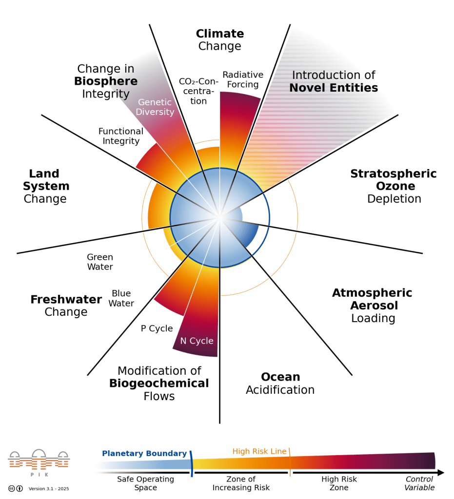
Planetary Boundaries¹⁹ ²⁰
Planetary Boundaries represent a framework identifying nine critical Earth system processes (climate change, biodiversity loss, ocean acidification, land system change, freshwater use, biogeochemical flows, ocean oxygen depletion, atmospheric aerosol loading, and chemical pollution) that regulate planetary stability. Crossing these boundaries increases risks of large-scale, abrupt, or irreversible environmental changes. The current status of the nine Planetary Boundaries is depicted in this visualisation by the Potsdam Institute for Climate Impact Research:

Planetary Boundaries visualised (this is the version for colour blind people)²¹

To understand why externalities pose existential threats, we must recognise that the Earth operates as a closed thermodynamic system. We receive energy from the sun, but practically no matter enters or leaves. The water, carbon, and minerals present today are the same atoms that existed millions of years ago. While companies test asteroid mining and space-based resource extraction, commercial operations remain infeasible. We are not going anywhere else, and neither is anything else any time soon.

Traditional economics assumes an implicit model of an open system where waste can vanish into a void without damaging the planet and new resources are in unlimited supply.²² ²³ Due to this, in traditional economics, environmental externalities don’t matter.²² In reality, extraction depletes stocks, and waste accumulates until organisms recycle it or it decomposes into usable molecules. This closed-loop reality means that all environmental externalities eventually cycle back, imposing costs on the system that produces them.

Ecosystems provide services worth far more than human-created capital. The real economic value of ecosystem services includes provisioning services (food, water), regulating services (carbon storage, water purification, disease control), supporting services (nutrient cycling, pollination), and cultural services (aesthetic, recreational, spiritual value). These services are valued at over $150 trillion annually, which is approximately twice global GDP, yet most remain invisible to the financial market.²⁴

When ecosystems collapse from pollution or overexploitation, the cascading effects are severe. Freshwater species populations have declined by 83%²⁵ in fifty years. Research demonstrates that losing 40% of key species can trigger collapse of 40% of remaining species throughout the system: ecosystems don’t gradually decline but flip to new, often irreversibly degraded states.²⁶ ²⁷ These ecological transformations represent enormous negative externalities that the economic system counts at no cost for the polluter.

Regime Shifts
When a planetary boundary is crossed, the Earth system risks undergoing a regime shift—an irreversible transition to a new, less hospitable state.

Systemic Financial Risk: These physical risks are becoming material financial risks. Current projections suggest that unmitigated boundary breaches could cause profit losses of 5-25% by 2050 for unprepared sectors. More dangerously, the “tipping point” in nature creates a “tipping point” in the economy, where insurance markets fail because risks become uninsurable (e.g., no one will insure property in a zone of permanent wildfire).²⁸
Non-Linear Damages: Traditional Cost-Benefit Analysis (CBA) struggles here because it assumes linear damages (e.g., 2 degrees of warming is twice as bad as 1 degree). However, crossing a tipping point (like the collapse of the Amazon rainforest or the West Antarctic Ice Sheet) causes damages to spike asymptotically to infinity, representing an existential threat rather than a marginal cost.²⁹

The efficiency trap³⁰ ³¹
In 1865, economist William Stanley Jevons observed a counter-intuitive trend in his book The Coal Question: James Watt had introduced a vastly more efficient steam engine that required less coal to do the same amount of work. Logic suggested that coal consumption would drop. Instead, it skyrocketed.

This is the Jevons Paradox: Because the new engine made energy cheaper, making it profitable to use steam power in thousands of new applications where it was previously too expensive. Increases in efficiency often lead to increases in overall consumption, rather than decreases.

Circularity
If Earth is a closed system, our economy must become one too. The circular economy is a fundamentally different way of thinking about production and consumption. Instead of extracting → making → disposing, the circular model aims for continuous circulation.

The Ellen MacArthur Foundation, which pioneered much of the circular economy theory, defines it as follows: “A circular economy is an economic model aimed at minimising waste and maximising resource efficiency. It focuses on reusing, repairing, refurbishing, and recycling existing materials and products to create a closed-loop system that reduces impact on the environment.”³²

At its core, the circular economy operates on a radical premise: there is no such thing as waste. Circularity isn’t just about recycling more; it’s about redesigning civilisation so that the concept of “waste” becomes obsolete. It mimics biological cycles where the waste of one species becomes food for another.

The more traditional concept of the circular economy rests on three complementary principles, often called the “Three Rs”:³³ ³⁴

Reduce: The most fundamental principle. Use less. Design products that require fewer materials. Choose quality over quantity. The environmental benefit of not using a material in the first place is greater than the benefit of recycling it later.
Reuse: Keep products in use for their original purpose as long as possible. A bottle is reused for storage. Clothing is worn by multiple people across time. Furniture is repaired and maintained rather than discarded when fashion changes. Reuse requires durability—products must be built to last.
Recycle: When a product reaches the end of its useful life, its materials are recovered and transformed into new products. But recycling is the least preferred option in the circular model, coming only after reduction and reuse. Why? Because recycling requires energy, and recycled materials often degrade in quality (a process called “downcycling”).

However, there are other Rs too:³⁵ ³⁶ ³⁷

Refuse: Refuse to buy what is not required.
Repair: To repair is to fix something that is broken and return it to working condition, and it extends products’ lives.
Refurbish: Refurbishment is the professional process of restoring a used product to like-new condition through cleaning, testing, repair of worn components, and quality assurance.
Remanufacture: Remanufacturing is the industrial process of returning end-of-life products to like-new condition, often exceeding new product quality. Unlike refurbishment (which typically involves minor repairs and cosmetic restoration), remanufacturing involves complete disassembly, assessment of every component, replacement of worn parts, cleaning, reassembly, and testing.
Recover: Resource recovery is the process of extracting materials from used products and waste, converting waste into valuable inputs for manufacturing new products. Instead of garbage going to landfills, its materials are recovered and re-entered into production cycles.
Regenerate: Regeneration is the final and highest aspiration of circular economy: not just reducing harm, but actively improving ecosystems, building natural capital, and leaving the world richer than you found it.

Circular principles include design for durability and repairability to extend product lifespans, material selection to enable recycling, take-back programs where manufacturers manage end-of-life, and remanufacturing to extract value from used products.³⁸

Industrial ecology formalises this concept by analysing material and energy flows through industrial systems. The goal is to create industrial ecosystems where output from one facility becomes input to another, mimicking natural food webs where energy and matter cycle through trophic levels. Successful industrial ecology requires partnerships among industries to exchange byproducts and shared infrastructure for waste processing.³⁹

The transition from linear to circular creates fundamental business model changes. Instead of maximising production volume, circular firms optimise product lifespan, material recovery, and service delivery. Instead of profit from disposal, revenue comes from extended use and material recapture.³⁸

From an environmental economics perspective, the circular economy represents internalising all externalities by forcing companies to account for their entire product lifecycle. When manufacturers know they’ll eventually manage end-of-life—or when cost of future pollution regulations is incorporated into today’s decisions—they’re incentivised to eliminate waste at design stage rather than manage it at disposal stage.

Pricing Nature
To fix the market failure, we first need to measure the damage. Forcing the market to account for costs previously external-to-firm decision-making by making polluters pay for environmental damage, market prices finally reflect true social costs. This can occur through multiple mechanisms: taxes, regulations, cap-and-trade systems, liability rules, or disclosure requirements. When externalities are internalised, the price of polluting goods rises to reflect their true cost.⁴⁰

The foundational principle that whoever causes pollution or environmental damage must bear the cost of preventing, mitigating, and repairing that damage is called the Polluter Pays Principle (PPP). Formally articulated by the OECD in 1972 and incorporated into the Rio Declaration in 1992, PPP creates economic incentives for polluters to reduce their damage. It shifts responsibility from the public (who would otherwise pay cleanup costs) to the private parties who profit from pollution.⁴¹ For this, we first need to be able to find the monetary value in question:

Replacement Cost Method:⁴² A valuation approach that estimates the value of an ecosystem service by calculating what it would cost to replace that service with human-made technology. For example, if replacing a wetland’s filtration service with a treatment plant costs $2 million, the ecosystem service is valued at $2 million.
Direct Valuation:⁴³ A method that estimates environmental value by asking people how much they would be willing to pay for environmental improvements (like cleaner water) or willing to accept as compensation for environmental losses. For example, surveys can estimate how much people value a protected forest by asking their willingness to pay for conservation. This captures existence value—what people value simply knowing something exists, even if they never use it.
Hedonic Pricing (Indirect Valuation):⁴³ A method that estimates the value of environmental attributes (clean air, clean water, scenic views) by analysing how they affect market prices. For example, homes near clean lakes or parks sell for more; the price difference reflects the value of the environmental amenity.
Travel Cost Method (Indirect Valuation):⁴⁴ A method that estimates the value of environmental amenities (national parks, beaches, forests) by analysing how much people spend to visit them. The travel costs (fuel, lodging, time) are used as a proxy for environmental value.
Avoided Cost Method:⁴⁵ A cost-based valuation approach that estimates ecosystem service value by calculating the costs that would be incurred if those services were lost. For example, the value of wetlands for flood protection can be estimated by calculating the property damage that would occur without the wetland’s protection.

Internalisation
After we’ve found the cost of pollution, the next step (once politically convenient) is to internalise the costs to those who pollute. This part of the post discusses some accepted measures.

1. Tax-Based Instruments⁴⁶ ⁴⁷ ⁴⁸
Pigouvian taxes, named after the previously-mentioned economist Arthur Pigou, are a direct approach to internalisation. A Pigouvian tax sets a fee equal to the marginal (in economics, marginal means additional) external damage at the socially optimal output level. For example, a carbon tax places a cost on CO2 emissions equivalent to climate damages. This transforms polluters’ incentives: with the tax in place, reducing emissions becomes cheaper than paying the tax, so firms invest in efficiency and cleaner technologies.⁴⁹

The advantage of Pigouvian taxes lies in flexibility. Rather than mandating specific pollution control technology, taxes allow firms to find the most cost-effective way to reduce emissions, whether through process changes, technology adoption, or output reduction.

However, implementing Pigouvian taxes presents challenges. Accurately estimating the monetary value of marginal external costs proves extremely difficult, particularly for long-term, diffuse environmental impacts like climate change. Additionally, poorly designed taxes can be regressive, disproportionately affecting low-income households. Well-designed tax systems can mitigate this through revenue recycling (using tax revenue to fund renewable energy research, reduce other distortionary taxes, or provide carbon dividends to citizens).

The double-dividend hypothesis suggests that revenue-neutral substitution of environmental taxes for income taxes yields two benefits: a better environment (the first dividend) and a more efficient tax system by reducing distortionary income taxation (the second dividend).⁵⁰ ⁵¹ While theoretically appealing, empirical evidence shows mixed results depending on multiple economic and policy factors.⁵⁰ ⁵¹

2. Cap-and-Trade Systems⁴⁸ ⁵² ⁵³ ⁵⁴
Cap-and-trade (also called Emissions Trading Schemes or ETS) represents an alternative market-based approach to internalisation. Regulators set a total cap on allowable emissions and distribute permits to polluters either for free or through auction. Firms must either reduce pollution or buy additional permits from other firms. Crucially, the cap declines over time, forcing progressively stricter emissions reductions.

The trading mechanism generates a two-fold benefit. First, companies that can reduce emissions cheaply have financial incentive to do so, then sell surplus permits to polluters facing higher abatement costs. This ensures that emissions reductions occur where they’re cheapest—society achieves the environmental target at minimum economic cost. Second, as the cap tightens, permit scarcity increases, creating financial pressure for innovation and investment in clean technologies.

Comparing cap-and-trade to carbon taxes reveals important trade-offs. Cap-and-trade provides environmental certainty—the government guarantees a specific pollution level through the cap—but costs fluctuate with market conditions. Carbon taxes provide cost certainty—polluters know exactly what they’ll pay per unit—but environmental outcomes depend on market responses. Under uncertainty about abatement costs, taxes work better when marginal benefits are relatively flat; cap-and-trade works better when they’re steep.

Cap-and-trade faces political and practical challenges. It requires sophisticated bureaucratic capacity to determine which companies get covered and how many permits to allocate. The system struggles to cover small polluters as only large facilities typically participate while taxes apply at the emission source (fuel) and thus reach both small and large users. Additionally, international trading risks creating environmental “hot spots” where permits concentrate pollution in particular locations, raising environmental justice concerns.⁵⁵

India’s approach offers a developing-country model. India’s Carbon Credit Trading Scheme, notified in 2024-2025, uses an intensity-based baseline-and-credit system covering nine energy-intensive industrial sectors. Entities that overachieve their emissions intensity targets earn Carbon Credit Certificates; those falling short must purchase or surrender certificates. The scheme also includes a voluntary domestic crediting mechanism allowing non-covered entities to register emission reduction projects.

3. Extended Producer Responsibility⁵⁶ ⁵⁷ ⁵⁸ ⁵⁹
Extended Producer Responsibility (EPR) shifts waste management liability from governments to manufacturers. By holding producers responsible for their products’ entire lifecycle—from material extraction through end-of-life disposal—EPR incentivises design changes that reduce waste at source.

Under EPR, manufacturers can implement reuse, buyback, or recycling programs, or delegate responsibility to Producer Responsibility Organisations (PROs) paid for used-product management. This shifts the burden from government to private industry, obliging producers to internalise waste management costs in product prices and ensure safe handling.

EPR functions as a powerful design incentive. When manufacturers know they’ll pay for disposal, they redesign products to use fewer materials, improve recyclability, avoid toxic substances, and extend product lifespans. Successful EPR implementation requires clear regulations defining which products are covered, what producers must fund, and how compliance is verified.

4. Market-Based Instruments Compared60 61
Research comparing different internalisation mechanisms reveals nuanced trade-offs. Market-based instruments (taxes, permits, subsidies) achieve environmental goals by altering the fundamental market framework and letting firms minimise costs. Choice-based instruments (eco-labels, voluntary certifications) let firms meeting criteria signal their qualifications to consumers, allowing consumers to express environmental preferences.

Empirical analysis shows that emission taxes prove more effective than voluntary environmental programs at enhancing environmental quality and welfare. While eco-labels capture additional consumer surplus from environmentally conscious buyers, taxation more effectively curtails emissions from inefficient firms by changing all firms’ incentives. Command-and-control regulation—mandating specific technologies or performance standards—typically costs more than market-based approaches but provides certainty about pollution outcomes.

In developing countries, command-and-control remains the predominant approach because regulations are easier to design initially using existing administrative apparatus. However, they often prove economically inefficient and prone to weak enforcement. Market-based instruments promise greater efficiency but require sophisticated governance structures, robust monitoring, and developed markets—typically scarce in developing nations. Effective environmental management likely requires hybrid strategies combining command-and-control for baseline standards with market mechanisms for achieving further improvements.

5. Command-and-Control Regulation⁶² ⁶³ ⁶⁴ ⁶⁵ ⁶⁶
Command-and-control regulation involves governments directly prescribing environmental standards and mandating compliance. The approach includes technology-based standards (requiring specific pollution control technologies), performance-based standards (setting pollution limits without specifying methods), and permits and licensing systems.

The clarity of command-and-control is its primary strength. Rules are explicit, leaving little ambiguity about compliance requirements. This predictability enables businesses to make precise investment decisions in pollution control. For regulators, assessment against specific benchmarks is straightforward.

However, command-and-control exhibits significant limitations. The uniform standards ignore that firms have different abilities to reduce pollution—what’s cheap for one firm may be prohibitively expensive for another. The approach provides no incentive to exceed standards, even if doing so would be cost-effective. Inflexibility about how to reduce pollution means the most efficient abatement pathways may be blocked by regulatory requirements.

Effective command-and-control requires strong institutional capacity for monitoring and enforcement. Many developing countries lack the resources for consistent inspection and credible penalties, enabling regulatory capture where polluting industries exert undue influence on regulatory bodies.

6. Information Disclosure as Policy⁶⁶ ⁶⁷ ⁶⁸
A third policy wave emerged beyond command-and-control and market mechanisms: information disclosure regulation. The U.S. Toxics Release Inventory (TRI), established in 1986 following the Bhopal industrial disaster, requires manufacturing facilities to publicly report annual toxic chemical releases to air, water, and land.

TRI operates on the premise that public information creates stakeholder pressure. When communities learn about facility emissions, they can pressure companies through reputation damage, consumer choices, or political action, creating incentives for pollution reduction without direct government mandates. The system is cost-effective because enforcement relies on stakeholder pressure rather than government agency capacity.

Research on TRI effectiveness reveals that responsiveness to disclosure varies. Establishments located near corporate headquarters perform better than isolated facilities, suggesting that internal expertise access and sensitivity to reputation in areas with multiple company facilities enhance response. Facilities far from headquarters, large plants in rural areas, or isolated operations may need additional incentives or resources to improve in response to disclosure alone.

7. Voluntary Environmental Standards⁶⁹ ⁷⁰ ⁷¹ ⁷²
Voluntary environmental standards represent commitments organisations adopt beyond legal requirements. These range from ISO 14001 environmental management systems certification to sector-specific standards like Forest Stewardship Council (FSC) certification for forests or Marine Stewardship Council (MSC) for fisheries.

Credibility requires external verification by independent third parties. This process adds weight to environmental claims and provides assurance to stakeholders that standards are genuinely met. However, voluntary standards face limitations: they reach only willing participants; stringency varies across programs, creating opportunities for firms to “venue-shop” across programs requiring lower standards; and participation often hinges on credible threats of future mandatory regulation rather than genuine environmental commitment.

Empirical research on FSC and similar standards reveals mixed outcomes. While standards aim to promote sustainable practices, effectiveness varies across global contexts, with weak governance structures and social capital challenges limiting success in some regions.

8. Payments for Ecosystem Services⁷³ ⁷⁴ ⁷⁵
Payments for Ecosystem Services (PES) represent a market-based approach to conservation. PES schemes compensate farmers or landowners for managing land to provide ecological services—carbon sequestration, watershed protection, biodiversity conservation, pollination services. A transparent system offers conditional payments to voluntary providers who maintain ecosystem functions.

PES advantages include cost-effectiveness. By offering fixed payment for service provision, individuals who can provide the service at or below that price have incentive to enroll, while those with higher opportunity costs do not. This self-selection ensures cost-effective service provision relative to mandatory approaches requiring same actions from all.

However, PES faces challenges, particularly for public goods. When ecosystem services benefit society broadly (like climate stability), individuals lack financial incentive to provide them without compensation. Converting latent demand into actual funding requires compulsory mechanisms—taxation or government payment—to overcome free-rider problems. Additionally, PES programs raise concerns about commodification of nature, potentially privatising commons and reducing indigenous land rights.

9. Mitigation Banking and Conservation Offsets⁷⁶ ⁷⁷ ⁷⁸ ⁷⁹ ⁸⁰ ⁸¹
Mitigation banking provides another market-based internalisation mechanism. Under the U.S. Clean Water Act Section 404, developers cannot discharge pollutants into waters without compensation. Rather than each developer creating individual compensatory mitigation, centralised mitigation banks allow developers to purchase credits from banks that restore or preserve wetlands or streams elsewhere. Before a 404 permit is issued, applicants must first avoid and minimise impacts; any remaining unavoidable impacts must be offset through compensatory mitigation, which can be accomplished via permittee‑responsible mitigation, in‑lieu fee programmes, or purchasing credits from a mitigation bank. Mitigation banking has evolved as an alternative to project‑by‑project mitigation, allowing developers to buy credits from centralised banks that have already carried out restoration/enhancement activities, which can be faster and administratively simpler for permittees.

This system incentivises restoration over preservation. Mitigation banking regulations reward restored wetlands with more credits than preserved ones, reflecting greater ecological value from restoration. Developers benefit from faster, cheaper compliance; ecosystem managers benefit from predictable funding for restoration; communities benefit from ecosystem protection even if harm occurs elsewhere.

Mitigation banking principles extend to conservation more broadly. Tradable permits for endangered species habitat, conservation easements where landowners voluntarily limit land use in exchange for tax reductions, and habitat credits create markets in environmental services. These approaches rely on Coasean bargaining—if property rights are clearly defined and transaction costs are low, polluters and victims can negotiate mutually beneficial agreements without government intervention.

10. Liability Rules and Environmental Compensation⁸² ⁸³ ⁸⁴
Some jurisdictions implement strict liability for environmental damage, requiring polluters to pay compensation regardless of fault. This differs from fault-based liability requiring proof of negligence. The Polluter Pays Principle underpins this approach, making polluters bear responsibility for restoration, remediation, and third-party compensation.

India’s National Green Tribunal has developed frameworks for environmental compensation, imposing penalties on industries violating environmental regulations. Compensation includes assessment costs, restoration costs, and compensation for direct and indirect damages to human health, property, flora, fauna, and ecosystem functions.

A Contextual Note on Climate Justice
We cannot equate the carbon produced by a family burning wood to survive the winter with the carbon produced by a millionaire flying a private jet. One is a symptom of energy poverty and a lack of alternatives—a victim of the system. The other is a symptom of excess—a beneficiary of the system.

The poorest 50% of the world is responsible for 10% of global emissions while bearing the greatest harm from climate impacts.⁸⁵ ⁸⁶ Meanwhile, a private jet can emit 2 tonnes of CO₂ in a single hour, which is more than an average person in many developing nations emits in an entire year.⁸⁷ ⁸⁸ ⁸⁹ ⁹⁰ Treating survival emissions as equal to luxury emissions is morally corrupt.

Sources

Greenhouse gas emissions 101 – I

Before we begin, if you want to understand the general big picture about what climate is, Earth’s climate history, and/or about climate change, you can read this very comprehensive post.

A greenhouse is a structure, made of glass or plastic, which captures heat inside it so that it’s insides are warmer and drier than the atmosphere outdoors. Greenhouses are situated outdoors so they have a regular supply of sunlight. We’ve all experienced closed indoor spaces with glass façades that heat up due to receiving sunlight, and require specific cooling solutions that encourage air flow, or artificial cooling through air conditioners, such as sitting inside a car or a room with all its windows closed on warm days. These hot-car experiences are also due to the greenhouse effect.

This effect happens because sunlight, which is primarily composed of (a tiny amount of) ultraviolet (UV) light, visible light, and near-infrared (NIR) radiation, easily passes through greenhouse covers (glass or plastic) into the inside of greenhouse, where the objects, plants, and soil absorb the heat, and become warmer. These warmed up objects now radiate heat in the form of long-wavelength thermal infrared (IR) radiation, which, unlike the incoming shortwave radiation (UV, visible light, NIR) is absorbed into the greenhouse envelope (a building’s envelope is the skin of the building- all the outside walls). Since the building envelop has now absorbed the heat, the structure and its insides warm up and stay warm. In short: this effect allows heat energy inside, but doesn’t allow all of it to escape.¹ ²

Similarly, greenhouse gases are gas molecules in Earth’s atmosphere that absorb heat emanating from the planet’s surface- that is, they act sort of like the transparent skin of a greenhouse which absorbs heat so that the plants inside can be warm in cold weather.¹ ²

Here’s how it works: Solar energy travels through the atmosphere and warms Earth’s surface. As the planet radiates this heat back toward space, it does so primarily as long-wavelength infrared radiation, which is the same form of heat that gets trapped in a physical greenhouse. Greenhouse gases in the atmosphere absorb this infrared radiation. Instead of letting it escape to space, they re-radiate it in all directions, with much of it directed back downward toward Earth’s surface. This creates a second source of heating (the first being our Sun), amplifying the warming effect and keeping our planet warmer than it would otherwise be.¹ ²

A point to note is that in an actual greenhouse building, the warm air inside cannot mix with the cooler air outside it. Similarly, because there is nothing to mix with, the air inside the planet cannot be diluted with cooler air.

The greenhouse effect has directly caused life as we know it now to exist on this planet (other forms of life could still exist without it, who knows), as without this natural greenhouse effect, Earth would be a frozen, inhospitable world. Temperatures would average around -18°C instead of the habitable 15°C we currently enjoy.¹ ² But we’re now enjoying too much of a good thing, and the planet is now heating up more than is good for the life that evolved to live in it when the average temperature was the aforementioned the habitable 15°C: it’s not that no life will survive, it’s just that much of it won’t, leading to general ecosystem collapse, and life will be very uncomfortable for the humans who do make it to the hotter planet.³ ⁴ ⁵ ⁶ ⁷ ⁸ ⁹ ¹⁰

What does parts per million/ billion/ trillion mean?¹¹
ppm/ ppb/ ppt are notations scientists who study climate use to understand how much of the greenhouse gases in question is present in the atmosphere. Different greenhouse gases are measured in different units depending on their concentration levels. Carbon dioxide, which is relatively abundant in the atmosphere, is measured in parts per million. Methane, which exists in much lower concentrations, is measured in parts per billion. The most potent synthetic gases, such as the fluorinated gases like SF₆ and NF₃, are measured in parts per trillion, because even seemingly insignificant amounts have significant warming effects.

Besides, saying “the atmosphere contains 0.000194 of a percent of methane” is far less convenient than saying “the atmosphere contains 1,942 ppb of methane”.

Thus, if a scientist is measuring how many molecules of CO2 are present in our vast atmosphere, and if the atmospheric concentration of CO2 is measured to be 400 ppm, this means that out of every 1 million air molecules, 400 are CO2 molecules, and the remaining 999,600 molecules are other gases. The same principle applies to measuring ppb and ppt. The conversion between these units is the same as for regular numbers:

1 ppm = 1,000 ppb
1 ppm = 1,000,000 ppt
1 ppb = 1,000 ppt

Here’s how Global Warming Potential is measured¹² ¹³
GWP measures how much heat a greenhouse gas traps in the atmosphere typically calculated over a 100-year time horizon, in comparison to the amount of heat trapped in the atmosphere by CO2. It’s calculated by the Intergovernmental Panel on Climate Change (IPCC) based on the intensity of infrared absorption by each gas and how long emissions remain in the atmosphere. The unit of measurement is called Carbon Dioxide Equivalent (CO₂e).

Carbon Dioxide Equivalents (CO₂e) provide a standardised way to express the impact of different greenhouse gases using a single, comparable metric. CO₂e is calculated by multiplying the quantity of a greenhouse gas emitted by its Global Warming Potential. The formula is:

CO₂e = Mass of GHG emitted × GWP of the gas

For example, if you emit one million metric tons of methane (with a GWP of 30) and one million metric tons of nitrous oxide (GWP of 273), this is equivalent to 30 million and 273 million metric tons of CO₂, respectively.¹⁴

This standardisation is crucial for several reasons because it allows comparison across GHGs and amounts of emissions, so no matter the gas that has been emitted or the amount of it emitted, it is easy to understand for everyone the effect it will have on the planet. It will also help compare emissions reduction opportunities across different sectors and gases, and help compile comprehensive national and corporate GHG inventories that include all greenhouse gases. Essentially, it provides a common language for understanding greenhouse gas emissions.

Radiative Forcing Vs. GWP¹⁵ ¹⁶
Radiative forcing (RF) is a measure of how much a substance or factor disrupts the balance of energy entering and leaving Earth’s atmosphere. It is expressed in watts per square meter (W/m²), representing the amount of energy imbalance imposed on the climate system: it quantifies how much extra energy is being trapped in the atmosphere by a given agent (greenhouse gas, aerosol, or solar change). Therefore,

Positive radiative forcing = warming effect (energy trapped)
Negative radiative forcing = cooling effect (energy lost to space)

In comparison, GWP is a simplified index that converts radiative forcing into a single comparable number by expressing it relative to CO₂.

GWP = Total radiative forcing from 1 kg of substance over time horizon / Total radiative forcing from 1 kg of CO₂

This formula is asking if 1 kilo of a substance is released into the atmosphere, how many kilograms of CO₂ would produce the same total warming effect.

Radiative forcing tells you the immediate, direct physics of climate impact. It’s precise but complex because each substance has a different RF value. GWP is a policy-friendly simplification that lets users compare “apples to apples”, so that if 1 million tons of methane (GWP 30) are emitted, vs. 1 million tons of N₂O (GWP 273), it is instantly known that the N₂O causes ~9× more warming.

Let’s take a look at the main GHGs
You can read more about pollution (natural and anthropogenic here).

Carbon Dioxide (CO₂)¹⁷ is the most abundant and significant human-caused greenhouse gas, accounting for approximately three-quarters of all anthropogenic GHG emissions. Before the Industrial Revolution, atmospheric CO₂ concentration was about 280 parts per million (ppm). By May 2023, it had reached a record 424 ppm, which is a level not seen in approximately three million years. Aside from it’s abundance in the atmosphere, CO₂ is also a particularly concerning GHG because of its atmospheric persistence. While about 50% of emitted CO₂ is absorbed by land and ocean sinks within roughly 30 years, about 80% of the excess persists in the atmosphere for centuries to millennia, with some fractions remaining for tens of thousands of years. This means that the CO₂ we emit today will continue warming the planet for generations.

Methane (CH₄)¹⁷ is the second most important greenhouse gas after carbon dioxide. Although it exists in much smaller quantities than CO₂, methane is extraordinarily potent: one ton of methane traps as much heat as 30 tons of carbon dioxide.¹⁴

Methane is emitted from both natural and human sources. Natural sources include wetlands, tundra, and oceans, accounting for about 36% of total methane emissions. Human activities produce the remaining 64%, with the largest contributions coming from agriculture, particularly livestock farming through enteric fermentation (this is a digestive processes in ruminant animals where microbes in their gut ferment food, producing methane as a byproduct) and rice cultivation. Other significant sources include landfills, biomass burning, and fugitive emissions from oil and gas production (unintentional, uncontrolled leaks of gases and vapors that escape the control equipment, sometimes due to poorly maintained infrastructure).¹³

The good news about methane is its relatively short atmospheric lifetime of approximately 12 years. This means that reducing methane emissions can have a more immediate impact on slowing global warming compared to CO₂, even though its effects are less persistent over the long term.

Nitrous Oxide (N₂O), also known as laughing gas, is a long-lived and potent greenhouse gas with a Global Warming Potential 273 times higher than CO₂. It has an average atmospheric lifetime of 109-132 years.¹⁴

Nitrous oxide emissions come from both natural and anthropogenic sources. Major natural sources include soils under natural vegetation, tundra, and the oceans. Human sources, which account for over one-third of total emissions, primarily stem from agricultural practices—especially the use of synthetic and organic fertilisers, soil cultivation, and livestock manure management.¹³ ¹⁴ ¹⁷ Additional sources include biomass or fossil fuel combustion, industrial processes, and wastewater treatment.¹³ ¹⁴ ¹⁷

Fluorinated Gases¹⁸ represent a family of synthetic, powerful greenhouse gases including hydrofluorocarbons (HFCs), perfluorocarbons (PFCs), sulfur hexafluoride (SF₆), and nitrogen trifluoride (NF₃). These gases are emitted from various household, commercial, and industrial applications, particularly as refrigerants and in electrical transmission equipment.

While fluorinated gases are present in much smaller quantities than CO₂, methane, or nitrous oxide, they are extraordinarily potent. Some have Global Warming Potentials thousands of times higher than CO₂. For example, SF₆ has a GWP of 24,300, and some HFCs have GWPs exceeding 10,000. Additionally, many fluorinated gases have extremely long atmospheric lifetimes, ranging from 16 years to over 500 years for certain CFCs, meaning they persist in the atmosphere for decades or even centuries.¹⁴

Water Vapor (H₂O) is technically the strongest and most abundant greenhouse gas. However, its concentration is largely controlled by atmospheric temperature rather than direct human emissions. As air becomes warmer, it can hold more moisture, creating a feedback loop: warming from other greenhouse gases increases water vapor, which in turn amplifies warming. This makes water vapor a climate feedback mechanism rather than a primary driver of climate change.¹ ² ¹⁹

Greenhouse Gas	Atmospheric Concentration¹⁷ ¹⁸	Global Warming Potential (100-yr)¹⁴	Warming Contribution¹⁷	Primary Sources & Their Contributions²⁰
Carbon Dioxide (CO₂)	Pre-industrial: 280 ppm \| Current: 423.9 ppm (↑152%)	1 (baseline)	~74.5% of total GHG emissions; 42% of radiative forcing increase since 1990	Fossil fuel combustion: 74.5% of total – Electricity/heat: 29% – Transportation: 15% – Industry: 24% – Deforestation: 6.5-12%
Methane (CH₄) – non-fossil	Pre-industrial: 730 ppb \| Current: 1,942 ppb (↑166%)	27.0	~17.9% of total GHG emissions; 16% of warming from long-lived GHGs	Agriculture: 42% (livestock 27%, rice 9%) – Fossil fuel extraction: 23% – Landfills/waste: 16% – Natural wetlands: 36%
Methane (CH₄) – fossil*	—	29.8	—	Fossil fuel fugitive emissions from oil & gas systems and coal mining
Nitrous Oxide (N₂O)	Pre-industrial: 270 ppb \| Current: 338 ppb (↑25%)	273	~4.8% of total GHG emissions; third most important long-lived GHG	Agriculture: 74-75% (synthetic fertilisers 30-50% of agricultural emissions) – Industrial processes – Biomass burning
Water Vapor (H₂O)	Pre-industrial: 0-4% (variable) \| Current: 0-4% (variable), increasing 1-2%/decade	Not directly comparable (feedback amplifier)	41-67% of total greenhouse effect (but as feedback, not primary driver)	Natural evaporation from oceans/land – Acts as feedback amplifier (increases 7% per 1°C warming) – Not directly emitted by humans
Tropospheric Ozone (O₃)	Pre-industrial: 20-25 ppb \| Current: 20-100 ppb (varies by location)	Varies regionally	Third most important GHG after CO₂ and CH₄; significant regional warming	Not directly emitted – Forms from: NOx + VOCs + sunlight – Sources: Transportation, industry, biomass burning
HFC-134a	Pre-industrial: 0 ppt \| Current: 96.9 ppt	1,530	Part of 2.8% F-gases contribution	Refrigeration and air conditioning: largest use – Aerosol propellants – Foam blowing – Summer emissions 2-3× winter
HFC-23	Pre-industrial: 0 ppt \| Current: Low but significant	14,600	Highest CO₂-eq among HFCs despite low concentration	Byproduct of HCFC-22 production – Industrial processes
HCFC-22	Pre-industrial: 0 ppt \| Current: Declining post-ban	1,960	Part of declining HCFC contribution	Refrigeration/Air Conditioning: primary source (97% of HCFC use) – Being phased out under Montreal Protocol
HFC-152a	Pre-industrial: 0 ppt \| Current: 9.93 ppt	164	Part of 2.8% F-gases contribution	Aerosol propellants – Foam blowing – Refrigeration
Sulfur Hexafluoride (SF₆)	Pre-industrial: Near 0 ppt \| Current: 6.7 ppt	24,300	Part of 2.8% F-gases contribution; Highest CO₂-eq among all FGHGs	Electrical equipment: switchgear, transformers – Magnesium production – Semiconductor manufacturing
Perfluoromethane (CF₄)	Pre-industrial: 34.7 ppt \| Current: 76 ppt	7,380	Part of 2.8% F-gases contribution	Aluminum production – Semiconductor manufacturing – Small natural sources: ~10 tonnes/year
Perfluoroethane (C₂F₆)	Pre-industrial: Near 0 ppt \| Current: 2.9 ppt	12,400	Part of 2.8% F-gases contribution	Semiconductor manufacturing: 1,800 tonnes/year – Aluminum smelting
Nitrogen Trifluoride (NF₃)	Pre-industrial: 0 ppt \| Current: Growing	17,400	Part of 2.8% F-gases contribution	Semiconductor/electronics manufacturing – Flat panel displays
CFC-12	Pre-industrial: 0 ppt \| Current: Declining (banned)	12,500	Declining contribution; negative forcing from ozone depletion	Previously: refrigeration (primary), aerosols – Now banned; emissions from existing equipment
CFC-11	Pre-industrial: 0 ppt \| Current: Declining (banned)	6,230	Declining contribution; negative forcing from ozone depletion	Previously: refrigeration, foam, aerosols – Now banned; emissions from existing equipment/foams
Black Carbon (BC/Soot)²¹ ²²	Pre-industrial: Low natural levels \| Current: No direct measurement in ppm/ppb	450–900 (100-yr GWP)*	Second or third most important climate forcer after CO₂ in some regions	Diesel engines – Coal power plants – Biomass burning: wood, agricultural waste (67% of human emissions) – Residential cooking/heating – Wildfires – Ranking: Fossil fuel > biofuel > biomass burning
CFCs (Total)	Pre-industrial: 0 ppt \| Current: Declining overall	6,230–12,500	Negative forcing due to ozone depletion (cooling effect)	Banned under Montreal Protocol – Residual emissions from existing equipment/foams
HFCs (Total)	Pre-industrial: 0 ppt \| Current: 89 ppt total	164–14,600	~2.8% combined with PFCs and SF₆; grown 310% since 1990	Refrigeration/AC sector: largest source (replacing CFCs/HCFCs) – Increased 310% since 1990
PFCs (Total)	Pre-industrial: 34.7 ppt \| Current: 82 ppt total	7,380–12,400	~2.8% combined with HFCs and SF₆	Industrial processes – Aluminum production – Semiconductor manufacturing
HCFCs (Total)	Pre-industrial: 0 ppt \| Current: Declining	90–1,960	Declining; negative forcing from ozone depletion offset by GHG warming	Transitional CFC replacement being phased out – HCFC-22 and HCFC-141b represent 97% of HCFC use

Some important Greenhouse Gases and how they contribute to global warming. Specific GWP values come from IPCC assessments and may be updated as science advances.

Key:

ppm = parts per million; ppb = parts per billion; ppt = parts per trillion
GWP (Global Warming Potential) is measured relative to CO₂ over a 100-year timeframe (IPCC AR6, August 2024)¹⁴
F-gases (fluorinated gases) collectively contribute 2.8% of total greenhouse gas emissions but have grown 310% since 1990
Water vapor is technically the most abundant greenhouse gas but acts primarily as a feedback mechanism rather than a forcing agent
Black carbon is not measured in atmospheric concentration like other GHGs because it’s a particulate (soot) rather than a gas, and has a very short atmospheric lifetime (days to weeks). The GWP range reflects uncertainty in mixing state and location; IPCC AR6 provides radiative forcing (+0.44 W/m²) rather than a formal GWP.
*Methane split: IPCC AR6 differentiates between fossil and non-fossil methane due to different atmospheric fates. Use CH₄ non-fossil (27.0) for biogenic sources and combustion; use CH₄ fossil (29.8) for fugitive emissions from oil & gas and coal mining where the carbon is of fossil origin.¹⁴ ²³ This is because fossil methane (GWP 29.8) adds carbon that was locked underground for millions of years to the active carbon cycle, representing a net addition of CO₂ when oxidised, whereas biogenic methane (GWP 27.0) comes from carbon that was recently in the atmosphere (absorbed by plants, eaten by livestock, etc.), so its oxidation just adds back the same carbon that was already in the atmosphere until recently and there is no net addition in the long term.²⁴

Sources of GHG emissions

The Energy Sector is the largest contributor to greenhouse gas emissions, producing approximately 34% of total net anthropogenic GHG emissions in 2019.²⁵ Within this sector, electricity and heat generation are the single largest emitters, accounting for over 25% of global emissions, with coal-fired power stations alone responsible for about 20% of global greenhouse gas emissions.²⁶ In 2022, 60% of electricity in many countries still came from burning fossil fuels, primarily coal and natural gas.²⁷ And of course, energy underpins every other sector, whether through fuel for agricultural tractors, for building space conditioning, or any other mechanical activity.
Industrial activities come next at 24% of global emissions. These emissions are usually from one of two sources: energy consumption for manufacturing processes, and direct emissions from chemical reactions necessary to produce goods from raw materials.²⁵ ²⁸ Within industry, cement production and metal production, especially steel, are particularly emission-intensive.²⁸ Since 1990, industrial processes have grown by a massive 225%, the fastest growth rate of any emissions source, driven by rapid industrialisation in developing countries.²⁰
Agriculture, Forestry, and Land Use contributed approximately 22% of global emissions in 2019.²⁵ This is an interesting sector because it’s a major source of non-CO₂ greenhouse gases.²⁹ Agriculture is the largest contributor to methane emissions globally, primarily from livestock farming and rice cultivation, which occurs in flooded fields where anaerobic conditions produce methane.²⁹ The sector also produces significant nitrous oxide emissions, primarily from the application of synthetic and organic fertilisers to soils.²⁹ Additionally, deforestation and land-use changes release stored carbon when forests are cleared for agriculture or development.²⁹
Transportation accounts for approximately 15% of global emissions in 2019.²⁵ The vast majority of transportation emissions come from road vehicles (cars, trucks, buses, motorcycles, etc.) which rely overwhelmingly on petroleum-based fuels.³⁰ Aviation and maritime shipping also contribute significantly, with international aviation and shipping representing growing sources of emissions as global trade and travel expand.³⁰ Since 1990, transportation emissions have grown by 66%, making it one of the fastest-growing sources of greenhouse gases.²⁰ ³⁰ The sector’s heavy dependence on fossil fuels and the long replacement cycles for vehicles make it particularly challenging to decarbonise quickly.³⁰
And finally, Buildings, whether Commercial or Residential, directly contribute approximately 6% of global emissions through fossil fuels burned for heating and cooling, as well as refrigerants used in air conditioning systems.²⁵ However, when indirect emissions from electricity use are included, buildings account for a much larger share, which is about 28% in the United States, because buildings consume approximately 75% of electricity generated, primarily for heating, ventilation, air conditioning, lighting, and appliances.³¹ ³²

Sources

Financing Climate Solutions IV: Insurance

Economic and financial impacts of climate change
First, some explanations. In climate change contexts, economists use “Economic Loss” to mean the total monetary impact on communities, sectors, or entire countries, including uninsured damages and broader ripple effects.¹ ² Economic loss is further divided into two types of loss, pure economic loss and consequential economic loss.

Pure Economic Loss is financial harm that occurs without any associated physical damage to property or persons, such as when bad weather warnings keeping people away from events they would otherwise pay to attend.³ ⁴ Consequential Economic Loss is loss that happens as a consequence of that physical impact, even if not immediately obvious, for example if excessive rains damage a local shop, which then has to shut shop for repairs compromising sales for the period.³ ⁴

These distinctions matter because even when it is not immediately evident, climate change drives losses through the economy in multiple ways large and small. Think of unemployment in a region due to a climate exacerbated disaster such as a forest fire which burns down parts of a town or a city, let’s say some warehouses or farms burn down, not only are assets lost in such cases, so is future consumption due to loss in employment income for those who worked in those warehouses or farms. Further, not every loss is or can be insured, but losses such as those caused by consumption loss after considerable climate disasters tend to have ripple effects across economies with no clear physical starting point.

Financial Loss refers to losses in actual money or other financial instruments (for example unencashed cheques lost in a flood event). It’s a more direct concept and includes only what can be counted.² ³

Understanding these terms helps us understand the following statistics a little better, while also realising that they can never grasp the full magnitude of climate damages.

Economic losses from natural disasters totalled $368 billion globally, driven by hurricanes, severe storms, and record heatwaves. As mentioned, the first half of 2025 is trending higher. In India, climate disasters cost India over $12 billion in 2025, with floods and heatwaves hitting agriculture and productivity especially hard.⁵ Projections show GDP per capita losses could reach 2.13% by 2025 and exceed 25% by 2100.⁵ Indeed, if global warming reaches 3°C by 2100, cumulative economic output could shrink by 15–34%. The net cost of inaction translates to a loss equivalent to three times current global health spending by 2100.⁶

Insuring against climate risks helps manage losses from climate change impacts such as extreme weather events, floods, droughts, and tropical cyclones, as well as more mundane events like too much or too little weather that affect economic performance, such as agricultural output, disrupted sports matches, rained in vacation seasons, and so on. The costs and frequency of extreme weather events have soared, with $100 billion in insured losses recorded in the first half of 2025 alone,⁷ ⁸ which is 40% higher than the same period in 2024 and more than double the 21st-century average⁷.

Term	What it Means in Practice
Pure Economic Loss	Financial hit without physical damage—like lost ticket sales because a bad weather warning kept customers away, even if nothing broke.
Consequential Economic Loss	Costs that ripple out from a disaster—like lost income when a business shuts for repairs, or when workers lose jobs after a factory burns.
Financial Loss	Tangible money lost—cheques that float away in a flood, crashed stock market values, or direct property damage costs.

In summary

Risk
The standard formula for risk is: Risk = Probability × Impact, where probability is the simple likelihood of an event happening, like we studied in school (here’s a post that talks about probability in deeper detail), and impact is how severe the consequences of the event would be, if it were to happen.⁹

In practice, insurers and climate researchers use risk matrices or quantitative models to assess and rank multiple risks in order of urgency, severity and other metrics. The formula for these kinds of advanced risk models can substitute “probability” with metrics like frequency, exposure, vulnerability, or asset value, and here the formula can change to something closer to: Risk = Threat Frequency × Vulnerability × Asset Value.⁹ ¹⁰

Financial institutions increasingly conduct climate stress tests to assess resilience under various climate scenarios. These tests measure CRISK, which measures the expected capital shortfall under climate stress scenarios, and functions similarly to financial crisis stress tests but incorporating climate risk factors.¹⁰ During the 2020 fossil fuel price collapse, major global banks experienced substantial CRISK increases; Citigroup’s climate-related capital shortfall rose by $73 billion in 2020 alone.¹⁰

Stress testing involves three steps: measuring climate risk factors (often using stranded asset portfolio returns as transition risk proxies), estimating time-varying climate betas for institutions, and computing capital shortfalls under stress scenarios.¹¹

DON’T PANIC HERE’S AN EXPLANATION: It’s like asking, if climate disasters happen, how much trouble would this bank be in? A stranded asset portfolio is the collection of companies that the bank is lending to, or whose stocks it owns, that would suffer most if the world suddenly got serious about fighting climate change. From this we subtract the returns of some regular stocks so that we can isolate the impacts of climate change. So let us say an extreme climate event happens, and this portfolio crashes by 50% in market value (market value is the value the portfolio assets would get if sold in the open market). Climate beta is a way to understand how much the bank’s own share price responds to climate events, or to governments cracking down on transition sensitive industries that it owns in the stranded asset portfolio. If a bank has lent lots of money to an oil and gas company, it will have a higher climate beta. We use the share price of the bank because it provides a real-time, market-based reflection of how investors perceive the bank’s overall financial health and risk exposure, including its sensitivity to climate-related events, making it a practical and observable indicator for assessing potential future losses and calculating stress test outcomes, which basically means that markets process information faster than accountants. Continuing with our example, let’s assume the bank has a climate beta of 0.6. In extreme climate stress (50% fossil fuel portfolio crash), this bank’s stock price would fall by 30% (0.6 × 50%). The final step is to understand, if the worst possible climate scenario happens, how much money would the bank need to stay afloat, for which the following formula can be used: Capital Shortfall = (Minimum Required Capital that a bank must maintain as mandated by the government) – (Bank’s Remaining Equity After Climate Shock).

Another example: Portfolio crash = 50%, climate beta = 1.2, therefore the bank’s stock price crashes by 60%. Now suppose the bank has total assets (the market value of the loans it has given out, the shares it owns, and any other assets) of $100, and the government has said that at the minimum it must have 10% of this amount with it at all times (the bank cannot use this money), so 10% of $100 is $10. Now let us say that the same bank had $40 in equity share capital, but because the price of this $40 crashed by 60%, it is now only worth 40% × $40 = $16. Since the $16 > the $10 the government said the bank must always have, this bank is safe. It is easy to see that banks that have different combinations of numbers will have different results.

Climate risk is not an abstract concept any longer simply because it is happening all around us, and we’re all suffering from it (and also because financiers have made formulae). Areas that suffer frequent climate impacts, whether (hehe, weather) direct or indirect are likely to suffer more financial consequences and have poorer asset protection since insurers would prefer to limit losses.¹² ¹³ It just so happens that these geographies are also the previously colonised Global South now suffering from the extended consequences of colonialism and the industrial revolution they did not partake in.¹⁴ ¹⁵

In 2023, the global insurance protection gap reached 67%- only 33% of $357 billion in economic losses from natural hazards were insured.¹⁶ This gap widens dramatically in developing countries, most of which are the historically colonised nations, where less than 10% of disaster losses have insurance coverage;⁵ Africa insures merely 0.5% of climate-related losses.¹⁷ Without intervention, uninsured global losses could double to $560 billion annually by 2030.¹⁶ Regions may become effectively “uninsurable” as coverage becomes inadequate, inaccessible, or prohibitively expensive.⁹ Another relevant stat: research indicates each 1% increase in insurance coverage moves countries 5.8% closer to achieving Sustainable Development Goals.¹⁸ ¹⁹ ²⁰

The protection gap stems from multiple factors:

Unaffordable premiums: Rising climate-related losses push insurers to increase premiums to reflect heightened risk, further widening affordability gaps and leaving many unprotected.²¹ ²²
Insufficient local risk data: In many emerging markets and developing economies, hazard maps and exposure data are incomplete, outdated, or inaccessible, limiting confidence in risk assessment tools and complicating underwriting decisions.²¹ ²³
Lack of government coordination across ministries: Fragmented policy frameworks, inadequate integration of disaster risk management with financial protection strategies, and limited inter-ministerial collaboration obstruct the scaling of insurance solutions and premium support schemes.²¹ ²⁴
Inadequate domestic financial sector development: In many emerging economies results in underdeveloped insurance markets, limited technical capacity among insurers and supervisors, low financial literacy, and weak distribution channels. These structural weaknesses restrict both the supply of insurance products and the demand from potential policyholders, perpetuating the protection gap.21 ²⁵

Types of climate risk²⁶
Climate risk refers to the potential negative impacts on society, ecosystems, or economies resulting from climate change. These risks are typically grouped into three main categories: physical risks, transition risks, and liability risks.

Physical Risks: These arise from the direct effects of climate change and are further divided into two subcategories:
- Acute physical risks are event-driven, such as hurricanes, floods, wildfires, tornadoes, heatwaves, or intense storms. These can cause sudden and severe damage to property, infrastructure, and supply chains.
- Chronic physical risks develop over a longer time frame. These include rising sea levels, gradual increases in average temperatures, changes in precipitation patterns, persistent droughts, land degradation, water scarcity, and ocean acidification.
Transition Risks: These are risks associated with the shift to a low-carbon economy and include challenges related to changes in policy, technology, market preferences, and investments. Examples include regulatory changes (carbon pricing, emissions limits), sudden shifts in market demand (e.g., decline in demand for fossil fuels), technological disruption (rapid adoption of renewables), or reputational damage if organisations are slow to adapt. Such changes may render some business models or assets less viable or even obsolete (these are called “stranded assets”).
Liability Risks: These stem from parties seeking compensation for losses they attribute to climate change. As regulatory requirements around disclosure and climate responsibility tighten, companies face increasing legal actions over failure to adequately manage or disclose climate risks, or for contributing to environmental harm.

More about stranded assets: To limit warming to 1.5°C, approximately 60% of oil and gas reserves and 90% of coal reserves must remain unburned, creating potentially $1.4 trillion in stranded fossil fuel assets globally.²⁷ Coal-fired power plants face the highest stranding risk, requiring retirement 10-30 years earlier than historical patterns to meet Paris Agreement targets.²⁸ Stranding extends beyond fossil fuels—aviation, heavy manufacturing, and carbon-intensive real estate also face obsolescence as the economy decarbonises. Physical climate risks like sea-level rise, floods, and droughts can also directly strand assets by making them uninhabitable or uneconomical. Buildings failing to meet emerging energy efficiency standards face early economic obsolescence, requiring costly retrofits or suffering reduced marketability.

The financial industry’s exposure to climate change¹⁰ ¹¹
The financial industry is exposed to climate risks on both sides.

In finance, buy side and sell side refer to the two broad categories of financial market participants and their roles in the investment ecosystem. The buy side includes entities whose primary role is to invest capital (money) for themselves or their clients, and their main goal is to generate positive returns from the purchase and management of these assets. Sell side entities provide investment products, research, and execution services to buy-side clients and often facilitate transactions between buyers and sellers.

Buy side entities face climate risk in the form of:
- Asset Value Declines: Physical climate events can damage or destroy underlying assets (like real estate, farmland, or infrastructure), eroding the value of investments.
- Transition Risks: As economies move to lower-carbon models, the value of companies or sectors exposed to fossil fuels, heavy industry, or outdated technologies may collapse, turning previously valuable holdings into “stranded assets”.
- Market Volatility: Unexpected regulatory policy, carbon pricing, or shifts in investor preferences can result in sharp drops in certain securities, particularly where climate risks were previously underpriced, or even unpriced.
- Reputational and Compliance Pressure: Asset managers are increasingly required to disclose their climate risk exposures, scenario analysis, and decarbonisation strategies under frameworks such as TCFD, EU taxonomy, and other local regulations.
And Sell side entities face them in the form of:
- Credit Risk and Loan Defaults: Borrowers struck by climate disasters (flood, drought, hurricane) may default on loans as asset values drop or cash flow dries up. Large-scale disasters can lead to significant concentrations of defaults in a short period.
- Collateral Devaluation: The value of physical collateral backing loans (properties, crops, factories) declines with repeated climate events or chronic risks such as sea-level rise or desertification.
- Underwriting Risk: Insurers see more frequent and severe claims for natural disasters, complicating pricing and threatening profitability.
- Rising Compliance and Capital Costs: Regulators increasingly require sell side firms to conduct climate stress tests, manage exposures, and allocate more capital against climate-vulnerable loans or portfolios (so that if their value suddenly declines, there is enough money to cover for it).

Some of the newer insurance instruments

Traditional vs. Parametric Insurance:¹⁰ Traditional indemnity insurance requires extensive damage assessment and claims verification, causing significant delays when communities need immediate relief. Parametric or index based insurance (called so because payouts are triggered by weather indices that measure heat waves, number of rainy days, wind speeds, etc.) trigger automatic payouts when predefined thresholds are met.

For example, if wind speeds in an area exceed 150 km/h, it may immediately send money to the people who are insured in that area, if rainfall below 200mm happens during growing season in an area, automatic payout will happen in that area, as long as data confirms that the threshold criteria were met. This brings transparency, expedites claims processing, and provides policyholders discretionary use of funds for their most urgent needs. Parametric insurance is also expanding to cover urban businesses, tourism, and logistics.

Catastrophe Bonds (CAT Bonds):²⁸ Catastrophe bonds are alternative risk transfer instruments that connect disaster risk to capital markets. Governments or corporations issue these high-yield debt securities through Special Purpose Vehicles, attracting investors including pension funds, asset managers, and hedge funds. Investors receive attractive returns—typically higher than traditional bonds—as long as specified catastrophes don’t occur. However, if predetermined triggers are met (a cyclone reaching specific intensity, earthquake exceeding certain magnitude, or insured losses surpassing threshold levels), investors forfeit some or all principal, which immediately transfers to the issuer for disaster relief and reconstruction.

The CAT bond market has grown substantially, reaching approximately $40-50 billion by 2025, up from minimal levels in the 1990s when they emerged after Hurricane Andrew devastated the insurance industry. India is exploring CAT bonds as the country faces $9-10 billion in annual disaster losses, with single events like the 2013 Uttarakhand floods causing over $6 billion in damages.

Risk Pooling Mechanisms:²⁹ ²⁶ Regional catastrophe risk pools aggregate disaster risks across multiple countries, exploiting geographic diversification where weather events affecting one nation are unlikely to simultaneously impact others. Research shows optimal regional pooling can increase risk diversification by 35-40% compared to individual country approaches. The three major global pools demonstrate this model’s effectiveness:

The Caribbean Catastrophe Risk Insurance Facility (CCRIF) covers tropical cyclones, earthquakes, and excess rainfall across Caribbean and Central American nations.
The African Risk Capacity (ARC) primarily addresses drought risk across African countries, with some coverage for other perils.
The Pacific Catastrophe Risk Insurance Company (PCRAFI) protects Pacific island nations against tropical cyclones and seismic risks.

These pools signed a Memorandum of Understanding at COP27 to collaborate on product development, advocacy, and capacity building.

Microinsurance for Climate Resilience:²⁹ Microinsurance extends risk coverage to low-income households in developing countries whose livelihoods are vulnerable to climate impacts. More than one billion unbanked adults live in the most climate-vulnerable countries, and they lack the financial resilience to withstand climate shocks.

Climate-linked index microinsurance products use satellite monitoring to trigger automatic payouts when drought, flood, or temperature indices reach predetermined levels, eliminating verification costs and fraud risks while providing rapid relief. Evidence suggests microinsurance helps vulnerable communities adopt risk management rather than harmful coping mechanisms after the events have happened, which then deepen poverty cycles.

Some microinsurance programs are now pairing parametric coverage against climate shocks with access to savings accounts or lines of credit accounts for post-disaster recovery. The idea is that this can strengthen community resilience.³⁰

Nature-Based Solutions and Insurance Innovation:⁵ Insurers increasingly recognise ecosystems2 as protective infrastructure deserving of coverage. Mangrove forests, coastal wetlands, and coral reefs provide natural storm surge barriers, while urban green spaces reduce flood risk and heat stress.

Insurance products now protect these natural assets and enable nature-based solutions, understanding that ecosystem degradation directly increases insured losses, although less than 2%²⁹ of international climate finance currently supports nature-based solutions for adaptation.

Instrument	What It Covers	How It Works	Who Uses It	Strengths	Challenges
Parametric Insurance	Weather extremes (rainfall, wind, drought, heat)	Policies pay out automatically if a set index (like rainfall, temperature) crosses a threshold—no need to prove physical loss	Farmers, governments, businesses in exposed areas, humanitarian agencies	Fast payouts, limited paperwork, works for hard-to-insure risks	May not match actual losses perfectly; needs reliable data
Traditional Insurance	Physical damage from weather/disaster	Payouts come after damage is verified, based on actual bills and assessments	Property owners, businesses, local governments	Familiar, covers wide loss types, can be customised	Slow response, costly verification, may not cover all gaps
Catastrophe Bonds (CAT Bonds)	Large-scale disasters (cyclones, earthquakes, floods)	Governments/businesses issue ‘high-yield’ bonds; investors lose their money only if disaster triggers payout	Countries, insurers, pension funds, asset managers	Brings capital markets into disaster relief, diversifies risk	Complex setup, investors risk losing principal if disaster strikes
Risk Pooling	Weather or disaster risks across regions or countries	Multiple countries/areas join a pool to share risks; one area hit, all pay, but events rarely hit all at once	Small nations, regional groups, insurance agencies	Reduces premiums, helps small countries access coverage	Governance is tricky, payouts depend on group solidarity
Microinsurance	Small losses for low-income, vulnerable groups	Ultra-affordable coverage, often parametric, sometimes bundled with savings, delivered by NGOs/banks/mobile	Farmers, informal workers, small businesses in climate hotspots	Swift and simple, increases resilience, avoids deep poverty	Can be less comprehensive, difficult to scale, requires outreach
Nature-Based/Ecosystem Insurance	Mangroves, reefs, wetlands, green urban assets	Policies protect/capitalise the restoration/maintenance of natural infrastructure	Coastal cities, local governments, conservation groups, insurers	Reduces cost of disasters naturally, preserves biodiversity	Not yet widespread, requires monitoring and valuation of natural assets

Comparable explanations of the different climate-related insurance products

In conclusion

As climate change intensifies, traditional insurance models face unprecedented challenges. Historical weather data, which is the foundation of actuarial science, becomes less reliable when climate patterns shift fundamentally.²⁶ Failure to manage climate risks exposes both buy and sell side firms to financial instability, reputational harm, and even legal action.

Financial institutions are adapting by increasingly adopting active risk management strategies that include scenario analysis, stress testing, enhanced data collection, and real-time monitoring of exposures to physical and transition risks, and by aligning governance structures, investing in climate modeling and reporting platforms, and embedding climate risk in all business decision layers including by setting climate-reduction targets, assessing financed emissions, and developing new risk-adjusted pricing and hedging strategies.

Sources

Emissions control technologies

What is Pollution?
“Pollution” is anything harmful or unwanted that has been added to the environment. Pollution makes the environment unsafe or unhealthy for living beings. It can take many forms: smog in the air, polluted rivers, plastic waste on beaches, excessive noise, or too much light that doesn’t allow us to see the night sky unhindered. Interestingly, pollution need not only be anthropogenic¹, although it usually is- examples of naturally originated pollution are ash from volcanic eruptions¹ ² exploding into the air around it, wildfires¹ ³ ignited by lightning causing smoke, ash, and burnt soil (in fact, air pollution can help wildfires create their own lightning and rain!!), dust storms⁴, sea spray (salt aerosols)⁵, pollen from plants⁶, radioactive gases from the earth like radon⁷, or even just the natural decay of organic matter⁸. A substance is categorised as a pollutant not by its origin, but by its effect- if it overwhelms nature’s ability to process or neutralise it, it is a pollutant.

Industrial vs. Natural Pollution
Industrial pollution comes from factories, power plants, and other places that make goods or energy. When these places take in raw materials (like oil, coal, metal, or chemicals) and turn them into products, the act of converting one product into another creates waste or toxins which are often released untreated into the environment in quantities the planet cannot naturally digest, and thus are left to infiltrate the natural world instead.

The planet has ways to cleanse itself—think forests soaking up CO₂⁹, wetlands filtering water¹⁰ ¹¹, or microbes breaking down organic matter¹²¹³. But when industries release more pollutants than the ecosystems can handle, several things happen¹⁴:

Bioaccumulation: Heavy metals and persistent toxins build up in soils, water, and living organisms, threatening animals and humans over time.¹⁴
Eutrophication: Nutrient pollution (nitrogen, phosphorus) from factories causes massive algae blooms in water, choking aquatic life.¹⁵
Smog and Acid Rain: Sulfur and nitrogen emissions react in the atmosphere, causing acid rain that harms forests and water bodies, and smog that damages lungs.¹⁶
Climate Change: Industrial greenhouse gases overload natural carbon sinks—heating the planet faster than forests or oceans can reabsorb emissions.¹⁷ ¹⁸ ¹⁹ ²⁰

Industrial pollution is quite different from pollution of a natural origin. For one, it’s caused directly by human activity, which means it often contains complex mixtures of artificial chemicals, persistent organic pollutants (POPs)²¹, heavy metals²³, synthetic compounds²², and engineered nanoparticles²². Many of these substances do not exist in significant quantities naturally and can remain toxic or disruptive for decades or centuries.¹⁸²⁴ Industrial pollution tends to be constant, widespread, and cumulative, with sustained emissions over years or decades (e.g., daily smokestack releases, persistent wastewater discharge), building up in our air, water, and soil to levels far beyond our home’s natural processing capacity, all of which creates long- term, regional, and global problems (e.g., acid rain, climate change, ocean acidification).¹⁸²⁴ Industrial pollutants are novel and often have no natural analogs, and can result in chronic overexposure for living systems.²²

In contrast, natural pollution, while hazardous, is typically more easily integrated or remediated by environmental processes, is episodic in nature, is naturally occurring and thus can be eventually reabsorbed by the Earth that produced it.²⁵¹

Treatment Technologies
There are a number of methods used to treat industrial pollution. Here’s a brief rundown:

1. Particulate Matter Control Technologies
Electrostatic Precipitators (ESPs)²⁶

How They Work: ESPs use strong electrical fields to “charge” tiny dust particles in factory exhaust. The charged particles are then attracted to plates with the opposite charge, sticking to them and leaving the air much cleaner.
Effectiveness: ESPs can remove up to 99.9% of dust and fine particulates—making them a powerhouse for cleaning industrial air, especially in power plants, steel mills, cement factories, and chemical works.
Variants: Dry ESPs: plates are shaken mechanically to dislodge and collect dust, Wet ESPs: Plates are sprayed with water, which continuously washes away dust.

Fabric Filters and Baghouses²⁷

How They Work: Picture a giant vacuum cleaner with hundreds of long, sturdy bags acting as filters. Dirty air passes through these bags; dust sticks to the fabric and forms a “dust cake.” It’s actually this cake that does most of the filtering.
Effectiveness: Baghouses trap over 99% of dust and even extremely tiny particles, outperforming most other dust controls for submicron pollution.
Cleaning Methods: Shaker: Bags are gently shaken to dislodge dust, Reverse Air: Air is blown backwards to release the dust, Pulse-Jet: Bursts of compressed air blast dust off the bags.²⁸

2. Gaseous Pollutant Control Technologies

Wet Scrubbing Systems²⁹

How They Work: Exhaust gases are washed or “scrubbed” with water or chemicals. Harmful gases dissolve in the scrubbing liquid or react to form “captured” compounds, which can then be removed.
Uses: These systems remove acid gases like sulfur dioxide, nitrogen oxides, and hazardous vapors in industries ranging from chemical plants to steel works.
Configurations: Venturi Scrubbers accelerate dirty air and spray it through water at high speed to trap both gas pollution and dust, Packed Bed Scrubbers pass polluted gas through a tower packed with materials (plastic, ceramic) to maximize contact with the scrubbing fluid, Spray Towers: Sprinklers ensure the widest possible liquid-air contact.
Benefits: Not only do wet scrubbers clear harmful gases from air, but they can also remove dust, cool hot gases, and help prevent fires.

Selective Catalytic Reduction (SCR)³⁰³¹

How They Work: SCR is the gold standard for cleaning nitrogen oxides (NOx) from exhaust. It injects ammonia or urea into hot industrial gases, which then react on a special catalyst to turn NOx into harmless nitrogen and water vapor.
Effectiveness: Can cut NOx pollution by 70-95%, which is crucial for power plants, ships, and large boilers.
Key Features: Requires careful temperature control (typically 180°C to 450°C) for best results, uses advanced catalyst materials (like titanium, vanadium, tungsten) for durability and performance in tough conditions.

Technologies for Volatile Organic Compound (VOC) Destruction
Thermal Oxidation Systems
How They Work: VOCs (volatile organic compounds) and other hazardous pollutants are destroyed by burning them at very high temperatures (around 1400–1600°F). The process breaks down harmful chemicals into carbon dioxide and water vapor.³²

Direct-fired oxidizers: Simple units that rely purely on heat.³³ ³⁴

Recuperative oxidizers: Use heat exchangers to recover energy for improved efficiency.
Effectiveness: When properly run, these systems can destroy over 99% of the target pollutants.
Safety & Control: Advanced thermal oxidizers continuously monitor temperature and emissions, shutting down automatically if anything goes wrong.

Regenerative Thermal Oxidizers (RTOs)³⁵

How They Work: RTOs take thermal oxidation a step further—they use beds of special ceramic material to trap and reuse heat, slashing energy costs.
Process: Air is directed through different sets of ceramic beds that absorb heat from outgoing clean air and transfer it to incoming dirty air, minimizing additional fuel requirements.
Effectiveness: Modern RTOs achieve up to 97% thermal efficiency and can sometimes run “fuel-free” if incoming air is rich enough in VOCs.

There are now also biological ways to treat the menace:

Biofilters: Air is pushed through beds filled with soil, straw, wood chips, or compost. Microbes living in the filter “eat” bad chemicals and smells (like VOCs—volatile organic compounds—from paint factories, food plants, or sewage treatments). The result is clean air and harmless byproducts.³⁶
Biotrickling Filters: Polluted air moves through towers packed with plastic or rock, sprayed with nutrient-rich water. Microbes grow on these surfaces. As the air flows, microbes capture and sponge up pollutants.³⁷ ³⁸
Bioscrubbers: Air is washed in tanks containing water and bacteria. Pollutants dissolve in the water, and the microbes digest them over time.³⁶
Industrial Wastewater Treatment with Microbes: Factories often create dirty water full of chemicals, oils, or heavy metals. Specialized treatment tanks use bacteria to eat these contaminants. Through activated sludge processes, millions of microbes clean water effectively before it’s released back to rivers or reused.³⁶

Industries often use layered strategies: A scrubber might remove much of the pollution, but a biofilter finishes the job, catching what remains.

Sources

Decarbonising the healthcare sector

I’ve unfortunately had a fair few run ins with the medical sector in India since 2023, and that has naturally made me curious about how it operates, especially from the point of view of decarbonisation (also, for anyone who is curious, the operation theatre I was operated upon in looked more like an enormous store room than what they look like in Grey’s Anatomy). Here’s what I found out.

The Sector
The healthcare sector is a sprawl of the multiple interacting industries, and includes healthcare providers (hospitals, clinics, nursing homes, physiotherapy), medical equipment & supplies (devices, diagnostic machines, consumables), pharmaceuticals & biotechnology (drug/vaccine makers, gene therapy, diagnostics), health IT & digital health (electronic records, telemedicine, AI platforms), managed Care/insurance (public/private health insurers, billing services), medical research & education (clinical trials, medical/nursing colleges, consulting), and ancillary/ wellness industries (medical tourism, public health, waste disposal). There’s also sectoral overlap with the real estate sector for the buildings these services are performed, or equipment manufacture at, supply chain and logistics, food and nutrition, and marketing.

So that’s a lot.

Global Statistics
All these industries accounted for approximately 10% of worldwide GDP- translating to nearly $10 trillion in health spending annually.¹ At the moment, the sector is the 5th largest emitter in the world, making for between 4.4% (2019) and 5.2% of total global greenhouse gas emissions currently¹ ², and might reach 6 gigatons by 2050 without aggressive decarbonisation efforts.¹ To help put this into perspective, 6 gigatons are 6,000,000,000 metric tons of carbon dioxide (CO₂). A typical passenger vehicle emits about 4.6 metric tons of CO₂³ per year, so the sector may emit as much as 1.3 billion passenger cars by 2050- and there are currently between 1.23 to 1.47 billion passenger cars in operation worldwide.⁴ ⁵

Before we go into the energy use, let’s understand how the emission break ups are categorised (Emissions are organised into three “scopes” to make it easier to identify where pollution comes from and how to address it): Scope 1 emissions are those emitted directly by the activities performed by the emitter, for example, the gas burned in your hospital’s boilers, emissions from ambulances and owned vehicles, or fumes from certain medical gases; Scope 2 emissions are indirect emissions related to the electricity, steam, heating, or cooling you purchase from someone else (like a utility company)- the pollution from this type of usage is created at the point of energy generation; and Scope 3 emissions are those not covered in the previous two, but are still only produced to be used in the healthcare sector- this makes it the trickiest and also the largest part of all the emissions from the sector- it includes the entire supply chain- so, for example, if a hospital buys a surgical kit, Scope 3 includes the emissions from making, packaging, and delivering it.

So now onto the break ups: globally these industries used 17% for Scope 1 emissions, 12% for Scope 2, and the remaining (71%) for Scope 3 uses in 2019.²

The India Story
The Indian healthcare sector made up 3.3% of national GDP as of 2022 (USD 80 per capita⁷), with expectations of this rising to 5% by 2030.⁶ India’s GDP in 2022 was approximately $3.35 trillion USD.⁸ ⁹ India’s total GHG emissions in 2022 were about 217.9 million metric tons CO₂ equivalent.¹⁰ 3.3% of National GHG Emissions (if scaled directly from GDP share) would be 217.9 million tonnes multiplied by 3.3%, or 217.9 multiplied by 0.033, which is approximately 7.19 million metric tons CO₂ equivalent (1,563,000 passenger cars). Actual sectoral emissions may vary depending on emissions intensity (a measure of how much energy is used to produce a unit of economic output). The Indian healthcare sector is estimated to account for about 2%¹¹ of national GHG emissions (4.36 million metric tons ÷ 4.6 ≈ 948,000 passenger cars), but if we scale strictly by GDP share (because there are no confirmed numbers), this figure is about 7.2 million metric tons CO₂e for 2022. I’ve also taken it as an equivalent percentage of GDP rather than the reported numbers because the Indian healthcare sector was estimated to emit 2% of India’s total GHG emissions in 2019², but between 2019 and 2022, the Indian healthcare sector grew by 17.5% annually¹², significantly outpacing the growth of the economy as a whole between these years⁸ ⁹. The healthcare sector’s 17+% CAGR versus the broader economy’s 7–8% CAGR means healthcare’s portion of the economy (and its GHG emissions footprint) increased during these years, likely easily outstripping the 2% estimate for 2019.

Decarbonisation Pathways

Why Is Healthcare So Carbon-Intensive? Because it uses a lot of energy, equipment, and material, many of which are:

Single-use: For sterility and safety, everything from syringes to gowns and often surgical tools are single-use. Single-use medical devices and consumables can account for up to 86% of the total carbon footprint of a hospital surgery, driven mostly by the production and use of such disposable items.¹⁴
Resource intensive: Hospitals need round-the-clock, energy-guzzling HVAC, lighting, emergency backup power, and sterilisation.²
Dependent on imports: Many hospitals, especially in countries like India, depend on imported medical technology, devices, and pharmaceuticals. The carbon footprint of these goods includes not just their production but also packaging, long-haul transport, and storage, increasing the indirect (Scope 3) emissions portion of healthcare’s footprint.¹⁵
Hazardous waste products: (e.g., sharps, blood-stained items, infectious waste) along with general plastic and food waste. Treatment and safe disposal—often via incineration—consumes a lot of energy and may itself release greenhouse gases and toxic substances such as dioxins and furans.¹⁶

Relationship between the healthcare system, climate change, and sustainability strategies and interventions. Source: The role of the health sector in tackling climate change: A narrative review – Zeynep Or, Anna-Veera Seppänen

A number of general and specialised strategies can be used to decarbonise operations in the healthcare sector.

General strategies (common to all energy users):

Transition to Renewable Energy: Switching to solar, wind, hydroelectric, and even geothermal sources for electricity, dramatically cutting GHG emissions. On-site solar photovoltaic (PV) installations, especially in hospitals, are reducing operational costs and increasing resilience.
Onsite energy generation: While not quire fully operational, or even fully sustainable yet, non renewable energy generation such as cogeneration or trigeneration, are certainly better than grid electricity usage as they will reduce transmission and distribution losses, and further the waste heat can be used to generate both heating and cooling, or both, for the premises.
Energy Efficiency Improvements: Upgrading and retrofitting buildings with energy-efficient lighting, HVAC (heating, ventilation, air conditioning), chillers, star-rated equipment, and insulation cuts down consumption by 30–50% in some cases. Use of variable frequency drives (VFDs)¹⁷, intelligent sensors, and IoT-based monitoring allows real-time optimization.
Green Building Design and Retrofitting: Buildings that follow green building codes and energy conservation codes consume fewer resources, while existing facilities can be retrofitted with modern energy management systems and green technologies.
Decarbonizing Supply Chains: Emphasis on green procurement, sustainable sourcing, and responsible supplier engagement ensures that scope 3 emissions are reduced and managed on an continuously.
Waste Management and Reduction: Sustainable waste handling, recycling, and waste-to-energy programs decrease landfill emissions and support circular economy practices.
Renewable or Low-GWP Refrigerants: A shift to low global warming potential (GWP) refrigerants to meet emerging regulations and climate commitments. (Global Warming Potential (GWP) is a measure of how much a greenhouse gas traps heat in the atmosphere compared to the same amount of carbon dioxide (CO2) over a specific time period, usually 100 years.¹⁸) Moving to refrigerants with GWPs far below 700 can cut emissions from these systems by as much as 78% (relative to older HFCs).¹⁹

Healthcare-specific strategies:

Low-carbon pharmaceuticals: Pharmaceuticals are among the highest-emitting components of healthcare’s carbon footprint, often due to energy-intensive manufacturing, complex supply chains, and waste at the point of use. A McKinsey study found that adopting green-chemistry principles to redesign synthetic processes and use recyclable solvents could cut pharmaceutical active ingredient (API) manufacturing emissions by up to 30%.²⁰
Reducing Low-Value Care: Avoiding unnecessary admissions, surgeries, and tests not only saves resources but reduces both direct (hospital-based) and indirect (supply-chain) emissions. Evidence-based guidelines to minimize unwarranted care can have substantial savings.²¹
Telemedicine and home- based care: Shifting care (where safe and appropriate) from hospitals to home or community settings lowers the need for energy-intensive infrastructure. For instance, remote physiotherapy after surgery demonstrated fewer rehospitalizations and better outcomes at lower environmental cost.²¹
Digistisation of care: Telehealth cut CO₂ emissions associated with cancer care by over 80% at one major U.S. center. Another 2023 multi-state analysis found telehealth averted 21.4–47.6 million kg of CO₂ per month—equivalent to keeping up to 130,000 cars off the road every month.²²
Treatments: Anaesthetic gases (like desflurane and nitrous oxide) have very high GWPs and alternatives (total intravenous or regional/local anesthesia) can be used where clinically appropriate without compromising treatment outcomes and patient health.²³

The healthcare sector is a vital, vibrant part of our world. It’s complexities and interdependencies make it difficult to decarbonise, not least that each decision should be made keeping patient service in mind, and at first it looks like decarbonisation does the opposite. Yet, we also know that climate change is making people sick: heatwaves, floods, wildfires, and storms are becoming more frequent and severe, and the World Health Organization (WHO) estimates that between 2030 and 2050, climate change will cause roughly 250,000 additional deaths per year from malnutrition, malaria, diarrhea, and heat stress alone- in some regions, heat-related deaths among people over 65 have risen by 70% in two decades²⁴; vector-borne diseases (like malaria, dengue, and Zika) are spreading to new areas as rising temperatures and altered rainfall enable disease-carrying insects to thrive in new regions and seasons, and water- and food- borne illnesses become more common when heavy rains, floods, or droughts contaminate water sources or affect food supply chains²⁵; rising air pollution including smog and higher particulate matter in the air we breathe smog and particulates), increases rates of asthma, chronic lung conditions, and cardiovascular disease affecting children, people with chronic illnesses, and urban residents are especially vulnerable; crop failures contribute to malnutrition and stunting²⁴ ²⁵; extreme events, displacement, and ecosystem loss contribute to greater rates of anxiety, depression, PTSD, and other mental health disruptions²⁶; rising seas, severe storms, and food/water shortages also force people from their homes, increasing displacement, conflict, and health emergencies- often overwhelming local health systems and worsening inequities²⁴… and working on sectoral decarbonisation will help those same people the sector works to protect.

Sources

Financing Climate Solutions – III: Weather or Climate Derivatives

A derivative is an asset whose value is based on a different underlying asset. They are called derivatives because they derive their value based on the value of something else. That something else is called the “underlying asset” and can be any asset, such as a stock/ share in a company, land, bags of grain, plant and machinery, inventory, or any other asset, group of assets, or even a benchmark¹, or a variable, such as the weather, or an event (outcome of an election). If something has an associated measurement that can be reliably quantified, it can be the “underlying asset”. The underlying asset is also called the “Primary Instrument”.¹

If there is any uncertainty about what the value of the underlying will be in the future, whether it is the price of a house, the earnings of a film, or how much rainfall there will be in the month of July next year, there can be a derivative about it. This is because derivatives are based on risk- some parties wish to protect themselves from a particular risk they foresee, and others believe that risk is worth taking. A derivative is a transaction between such risk averse/ risk protective and risk friendly parties.

Why do some people wish to take on more risk while others avoid it? Because humans have different opinions about what will happen in the future, generally believe they are correct about their assessments, and have varying risk appetites. Those with higher risk appetites may think of derivatives either as a wager, or a bet, and those with lower risk appetites may look at them as insurance or hedging against risk.

When thinking of derivatives as wagers or bets, we can liken them to sports betting, and just like organisations that run bets on sports matches have books of odds of what they think the result is likely to be, weather derivatives have an “index” of what is the normal or average or expected weather for a particular geography at a particular time of the year, and how likely it is to be that kind of weather. This is also called speculation- we are speculating on what the associated value measurement of the primary instrument will be at some point in the future, or, we are making a bet or a wager that it will be a particular value, but their value in climate finance lies in the security they provide against weather abnormalities. For example, both less and more rainfall than expected can be negative outcomes for farmers as both can ruin their crop. This sounds like an insurance, except that insurances pay out only when all their conditions are met- derivatives pay out when there is any deviation of the value of the underlying asset from what it was supposed, or expected, to be (the average value).

This is how derivatives can be used instead of insurance, and also why they are often considered better than insurance for those who know how to use them- insurance firms pay out only if there is evidence of a loss, and the loss must be proven to their standards, and even so your entire amount may not be covered due to contractual issues or because they don’t cover certain common types of losses, or even because the insurance company does not consider the evidence you provide to be sufficient. A derivative will pay out immediately as long as there is a difference between what was supposed to happen according to the contract, and what actually happened.

There are two general types of derivatives- firm commitments, and contingent claims. If parties participate in a firm commitment, that is, they promise, they must then fulfill the promise and complete the contract. For contingent claims, you have the option to follow through or not at the time the contract becomes due.

Because the value or price of the primary asset on which the derivative is based can move upwards or downwards, derivatives can also be thought of as being based on the direction of this movement. This is why some contracts are called “long” and some are called “short”:

Long contracts- you will benefit if the value of the underlying asset increases in the future. In case of sports for a match between Teams A and B for Team A to win, you are long (bullish) or you are long on Team A’s chances to win (winning being considered positive, generally).

Short contracts- You will benefit if the value of the underlying asset decreases in the future. In the case of the sports teams, since you are expecting Team A’s victory to take place, you will be short on Team B, because you expect their loss to take place or their value to decrease after the given match.

Example: Let’s say you come to know that Company X will purchase Company Y in the future, you are likely to purchase more shares of Company Y, because usually the purchasee is overvalued by the purchasing company, therefore the price of the shares of Y will increase since X is likely (via historical evidence) to have paid more for Y than Y is actually worth. Simultaneously X’s value is likely to reduce in the future because they have paid more than they should have. You are therefore long on Y and short on X.

Types of derivatives:

Futures

A Futures contract is an agreement to buy or sell an underlying asset at a future date and price that are both set down in the contract.

Futures contracts are standardised, and the counterparty is always the exchange it is traded on- this means, the entities buying or selling the contract do not have contact with the party selling or buying (respectively) the contract. Each party only interacts with the exchange on which the trade is taking place. Because they are exchange traded, the contracts are standardised rather than personalised.

These contracts are also settled daily by the exchange with the involved parties, so if the buying price of the contract increases, the exchange will ask the purchasing party to top up the difference, further discouraging rogue traders. Further, since these contracts are standardised and exchange traded, they are liquid and transparent.

Example: A natural dye trader worried that her crop of marigolds has not yielded enough flowers in time to make the dye for her next shipment due. She decides to purchase a futures contract for a few additional caseloads of fresh marigold petals, thinking that it’s okay if she ends up with more golden dye rather than less of it.

The contract states that two weeks from the date of purchase, the purchaser of the contract will pay the USD 150 for two kilos of fresh marigold petals. Now the farmer is certain that weather her farm produces enough marigold or not, she will have ready to use fresh petals for making her dye.

Let’s assume that on the date of delivery the price of two kilos of fresh marigold petals is USD 140 in the market, then the farmer still has to pay USD 150 for her delivery. And vice versa.

Forward

A Forward contract is similar to a Futures Contract, with the sole difference that these are customised private contracts between two parties rather than exchange traded.

Therefore these are not centrally settled, they are not liquid, and there is a possibility that the counterparty, which is the other trader and not a central exchange, may renounce the contract at any point, leaving the other party hanging.

Example: Morgan and Akanksha enter into a contract with each other to buy and sell 10 crayons of the now discontinued Crayola Daffodil Yellow. These are not available in the market any longer, and Akanksha is the only seller available, so she can decide any terms. This is also a very small quantity of product and an unusual product for the commodity markets. Morgan and Akanksha therefore enter into a Forward contract to accomodate all the unstandardised elements of their exchange.

If either party were to decide to dishonour the contract at any time before the exchange is completed, there would be no penalties exacted upon them, and the contract would fall through.

Options

Options, give people the possibility of doing something in the future. There are two kinds of options: A Put option, and a Call option.

A Put option is the right, but not the obligation (that is, the option), to sell an underlying asset in the future at a certain price which will be decided at the time of the contract.

A call is the right, but not the obligation, to purchase an underlying asset in the future at a certain price which will be decided at the time of the contract.

Example: A restaurant does not know how many tourists the city will host next year. Depending on whether more than expected tourists come, the owners of the restaurant wish to secure their supply of onions for their famous French onion soup. If there are more tourists, there will be more demand for onions, and then their prices will increase- and yet, the restaurant cannot always increase the price of the soup to reflect the increased price of the onions.

To secure their future supply, and to save themselves price uncertainty, they buy the option to buy more onions during tourist season at current prices. Now they are assured that if prices increase, or supply is tight, they will still have access to the produce. In case at the specified time the option can be exercised, the price of onions drops, they can always just buy from the market, and their only loss is a small fee paid to purchase the option, which for the restaurant is a call option.

If the market price of onions is higher than the price they agreed to pay as part of the Call Option they have bought (that is, they bought the option to buy onions), the restaurant can buy at the Call price and save money in comparison to what they would have paid for buying onions off the open market.

If the market price is less than the call price, they can just buy from the market and the only money they lose is the small amount they paid to buy the Call Option.

Example: For a Put Option, think of a scuba diving instructor, whose business is weather dependent, buys the Option to sell his lessons to a cruise shipping company. This is a Put Option, because it is the option to sell. If during the given week, the weather is good, the scuba diving instructor can sell his lessons at a higher price to other tourists and make more money. However if the weather is poor and tourists do not wish to go scuba diving, he can still sell to the cruise ship company.

Swaps

Swaps allow us to exchange cashflows.

Certain types of financial contract result in a stream of cashflows. For example, a debt contract results in a stream of interest income. Parties can agree to swap the interest they will receive (or pay) in the future with each other.

Example: In terms of climate financing, think of a weather dependent business, for example a movie shooting outdoors. The film production house can get into a Swap contract with a financing company. Let’s say the film company requires 20 continuous days of sunshine and warm weather at their location. They can get into a Swap Contract that says they require an average of 10 hours of sunshine daily, and another Swap that says they want an average of 25°C temperature daily for the twenty days of their shoot.

If the weather is different over the time period for which the film producing company bought the derivatives, they will automatically be paid (just by comparing the actual weather to the base index) and can use the money to cover additional costs that were incurred due to the different weather (like it was rainy instead of sunny).

So, a film production company (Party A) and a financial institution (Party B) enter into a weather swap that says that if there is more than 0 cm of rain between June 20 and July 10 at their location, Party B will pay $10,000 per day where there is more than 0 cm of rain to Party A.

Weather Swaps are generally two way contracts, so depending on the contract, perhaps if there are no rain disruptions, the Production Company may pay the financial institution $10,000 x 20 days = $200,000 instead. This depends on the contract they have entered into.

Sources

Understanding Derivatives: A Comprehensive Guide to Their Uses and Benefits

Financing climate solutions – II: adaptation finance

Climate change adaptation finance is the gangplank between addressing constantly escalating climate threats, and our current level of climate adversity preparedness- that is, it is used to help adjust to the adverse effects of climate change, such as floods, fires, or other extreme weather events.

The UNEP’s Emissions Gap Report 2024 states that while it remains technically possible to get on a 1.5°C pathway, a failure to deliver superior results would put the world on course for a temperature increase of 2.6-3.1°C over the course of this century.¹ To achieve the pathway to limiting temperature rise to 1.5°C, the current estimates are that the annual adaptation finance gap is US$187-359 billion per year², and developed countries, that did most of the climate damage must double adaptation finance to at least $40 billion a year by 2025³.

In 2022, the total financial flows to adaptation efforts were assessed to be $32.4 billion⁴, while another approximation puts this value at $63 billion⁵, which is nearly twice the first estimate- and yet, to put our requirements into further perspective, the all nations at COP29 agreed that the all sources of finances should generate $1.3 trillion annually by 2035, less than 10 years from now⁶.

Various financial mechanisms and instruments have been devised to address the gap. Here is a brief run down of some interesting ones:

1. Results based finance/ Outcome-Based Instruments- Money is paid out only once the previously agreed results are achieved. Debt-for-climate swaps/ Debt-for-Nature Swaps- “In a debt-for-adaptation swap, countries who borrowed money from other nations or multilateral development banks (e.g., the IMF and World Bank) could have that debt forgiven, if the money that was to be spent on repayment was instead diverted to climate adaptation and resilience projects.”⁷ These are a type of Results Based Financing.

2. Blended finance- The use of cataclytic finance to increase private sector participation in climate financing.⁸ Catalytic capital—debt, equity, guarantees, and other investments that accept disproportionate risk or concessionary returns compared to a conventional investment in order to generate positive impact.⁹ For example, guarantees are an assurance by a party that they will bear all losses for a project in case any occur, so that other investors come in to finance the project. Pooled investments are another example of blended finance, where capital from different entities is combined to finance projects.⁸

3. Payment for Ecosystem Services (PES)- The beneficiaries of ecosystem services remunerate those who tend to the ecosystem in question. A hypothetical example is paying the tribespeople who live in and tend to the Amazonian forests for providing a green lung to the rest of the world.

4. Liquidity facilities- Providing loans at the time of a crisis, often at concessional rates, or deferring repayments of old debts after an extreme weather event so that the nation(s) suffering from it have adequate liquidity to help their citizens.

5. Bonds- A bond is a debt instrument which offers an interest rate in exchange for lending money to the issuer of the bond. When the issuer is a sovereign, the interest rates are usually low since it is believed that they can cover at least the nominal value of the interest and the basic capital borrowed, whereas riskier debts such as corporations must offer more attractive rates of interest.

Catastrophe bonds are bonds issued to investors by insurers or pension funds which are offered at attractive rates and cover the risk of a climate catastrophe. In case such an event occurs, these funds are called in, however in case no such disaster happens, the investors benefit from the high interest rates.

There are also a variety of sustainable bonds, such as green bonds, sustainability-linked bonds, blue bonds, etc. and are used to fund different types of climate projects.

6. Green securitisation- Securitisation is the practice of clumping various financial instruments with similar characteristics together to form a completely new instrument which can then be sold to those willing to accept the risks and rewards associated with that new instrument, and the underlying securities. If the underlying securities were originally issued for climate friendly projects, they are called “Green Securitisation”.¹⁰

These and other mechanisms are all geared towards luring private funds into covering the gaping mouth of climate change adaptation requirements. Its clear that the need is dire, however these and other climate related mechanisms still form a tine part of the global capital markets.

Sources

The path to a just transition – II

In this part of the series of posts on a just energy transition, I’ll explore what an energy transition is, and why we must achieve it.

Energy transition is simply the switch our current dependence on fossil fuels to renewable or low carbon sources for energy production. This is essential because climate change is being fueled by our dependence on mineral fuels- the use of which release greenhouse gases into our atmosphere.

Greenhouse gases are gases that trap the Sun’s heat in our atmosphere, leading to a long term warming of our planet, causing local and global weather changes that living beings on the planet did not evolve with, and also causing abiotic planetary forces to react in ways that harm life and infrastructure- for example, warmer oceans lead to more hurricanes, causing greater property damage and loss of human, animal, and plant lives.

Since these gases collect in the atmosphere, there is a build up of heat absorbing chemicals in the air over time. Carbon Dioxide in particular persists in the atmosphere fore thousands of years, which means that the CO₂ released into the atmosphere by, for example, burning coal to fire steam engines during the industrial revolution, is still blanketing us today. Other gases issued due to the combustion of fossils have shorter lifespans, but greater warming effects due to the structure of their molecules- although methane (CH₄) on average lasts in the atmosphere for less than 12 years, it’s 100 year warming potential can be between 28 to 36 times as potent as CO₂, for example¹.

Just like if the planet were to cool (and continue cooling) overmuch, a planet that is heating up is catastrophic to life and property.

In comparison, non fossil sources of energy are considered clean fuels, since they do not liberate the greenhouse gas genie into our atmosphere while operating to produce energy. Please do note that while they contribute negligible amounts to global warming while making electricity, they do contribute to it through their supply chains- that is, scope 2 and 3 emissions.

The National Renewable Energy Laboratory (NREL) reviewed nearly 3,000 published life cycle assessment studies on utility-scale electricity generation
from wind, solar photovoltaics, concentrating solar power, biopower, geothermal, ocean energy, hydropower, nuclear, natural gas, and coal technologies, as well as lithium-ion battery, pumped storage hydropower, and hydrogen storage technologies, greenhouse gas (GHG) emissions from various sources of energy to inform policy, planning, and investment decisions. Less than 15% of the studies passed the various quality and relevance checks. On studying the ones that did pass these checks, NREL came to the conclusion that the Median Published Life Cycle Emissions Factors for Electricity Generation Technologies was as follows²:

S. No.	Type of Technology	Generation Technology	Median Published Life Cycle Emissions Factors
1.	Renewable	Biomass	52
2.	Renewable	Photovoltaic^a	43
3.	Renewable	Concentrating Solar Power^b	28
4.	Renewable	Geothermal	37
5.	Renewable	Hydropower	21
6.	Renewable	Ocean	8
7.	Renewable	Wind^c	13
8.	Storage	Pumped Storage Hydropower	7.4
9.	Storage	Lithium-ion Battery	33
10.	Storage	Hydrogen Fuel Cell	38
11.	Non Renewable	Nuclear^d	13
12.	Non Renewable	Natural Gas	486
13.	Non Renewable	Oil	840
14.	Non Renewable	Coal	1001

Median Published Life Cycle Emissions Factors for Electricity Generation Technologies
a Thin film and crystalline silicon; b Tower and trough; c Land-based and offshore; d Light-water reactor (including pressurized water and boiling water) only

As can be seen in the table above, the median Emission Factor (Emission Factors are a way to understand how much GHG emissions were released due to a particular activity) for the total lifecycle Non Renewables are far greater than those of either storage or renewable technologies. These emissions are primarily released during the combustion phase for the Non Renewables, however non of the other technologies require combustion to create electricity (and neither does Nuclear Light-Water Reactor technology, resulting in the very low Median Lifecycle EF).

Global greenhouse gas (GHG) emissions grew by 51% from 1990 to 2021, and more than 75% of these emissions come from the energy sector.³ Thus it’s obvious that by switching over to sources of energy that are not carbon intensive, we will be able to target the most conspicuous source of planet warming emissions. Shifting out of non renewable sources of energy will also reduce our dependence on fossils, and diversify our energy mix and enhance global energy security (in 2022 fossil fuels provided 81% of the total energy supply globally⁴), improve global health outcomes by reducing pollution, and finally- also improve the climate outlook.

Sources

Share this:

Share this:

Share this:

Share this:

Share this:

Share this:

Share this:

Share this:

Share this:

Share this: