Now you ask: “What is the chance that it rained, given that the ground is wet?”
That’s exactly the kind of question Bayes’ Theorem answers.
Think of Bayes’ Theorem as a smart way of changing your mind when new information appears. In life, we start with a belief based on past experience. Then something new happens. Instead of ignoring it, we usually update what we believe. It’s a part of Probability Theory that helps you combine old information you already have, with new information you have just received.
It looks mad, doesn’t it? It took me months to be able to remember the Bayes formula, and it took cricket to help me learn it finally. But first, an explanation of what we have above:
In the formula,
A = the thing you care about (Example: It rained). This is your starting belief before you see new evidence. It could be anything, such as, it’s dry season so it won’t rain today.
P(A) is the probability of the starting belief.
B = the evidence you see. (Example: The ground is wet). This is new information.
P(B) is the probability of the new information happening.
the “|” sign in the formula means “given” so P(A|B) will be read as Probability of A given B, meaning that the probability that A is still true given that the new information B is now known (“Now that I see the ground is wet, how likely is it that it rained?”), and P(B|A) is the probability that B is true given that we know that A happened (“If it did rain, how likely is the ground to be wet?”).
Now let’s take some help from cricket WITH MADE UP NUMBERS:
Let’s say India wins 70% of all cricket matches. This is P(A), where A = India wins 70% of all cricket matches, okay?
Now imagine Virat Kohli makes a century in 40% of the matches he plays. This is P(B), where B is Virat’s imaginary (I haven’t checked) century strike rate.
P(A|B) is the probability that India won a match given that Virat hit a century. Let’s keep this at 80%.Yes I’m a fan, how did you guess?
Now the new information is that India has won a match. So given that we now know that India has won a match, what is the probability that Virat hit a century?
So, now,
P(India winning a match for any reason) = 70% = 0.7
P(Virat’s century in a winning or losing cause) = 40% = 0.4
P(India winning given that Virat has hit a century) = 80% = 0.8
So, if we know India has won, what is the probability that Virat hit a century?
P(Virat’s Century given that India has won) = [P(Virat’s century in a winning or losing cause) × P(India winning given that Virat has hit a century)] / P(India winning a match for any reason)
I know this is all new and complex for many readers (it took me lots of effort and a Virat-inspired intervention to learn this too), so take your time to read it again if you need to, as many times as might help.
Player of Series Monsters At this point I want you to know that Cricinfo doesn’t have a list of women cricketers in decreasing order of player of series awards like they do for the men. There’s also a paucity of tabulated data available for women’s cricket generally. So I’m concentrating only on the men. The list of men is clearly documented, as mentioned:
Name
PoS Awards (Tests, ODIs, T20Is)
Virat Kohli (India)
22
Sachin Tendulkar (India)
20
Shakib Al Hasan (Bangladesh)
17
Jaques Kallis (South Africa)
15
David Warner (Australia)
13
Sanath Jayasuriya (Sri Lanka)
13
Of these, I got Perplexity AI to do some data finding and number crunching for me for Virat, Sachin, and Shakib for ODIs.
BayesUSING REAL NUMBERS When the team won, how often was this player the reason?
~24% of India ODI wins with him include a Kohli hundred
Tendulkar
India (ODI)
0.505
0.11
0.67
0.14 (14%)
~14% of India ODI wins with him include a Tendulkar hundred
Shakib
Bangladesh (ODI)
0.36
0.03
0.77
0.07 (7%)
~7% of all Bangladesh ODI wins include a Shakib hundred
Bayes calculation for Virat, Sachin, and Shakib
What this means
Virat Kohli in a strong India: One in every four ODI wins arrives with a Kohli century inside it. He does not just bat well; he bats well in a machine that is already built to win. His centuries are the accelerant on a fire that’s already burning. When India wins, there’s a strong chance he is the one who decided the margin, the pace, the emotional tone of the chase.
Sachin Tendulkar in a medium India: One in every seven wins contains a Tendulkar century. He played across eras—through the ’90s when Indian cricket was still finding its feet, through the 2000s when it became a force. His centuries had to do more heavy lifting because the team around him was less consistently dominant. The win probability bump he created had to be steeper, had to arrive at moments when India could genuinely lose without him.
Shakib Al Hasan in a historically weaker Bangladesh: One in every fourteen overall Bangladesh ODI wins includes a Shakib century—but here’s the insight: when he does score a hundred, Bangladesh almost never lose that game (6 of 7). On a much thinner winning base, his performances are load‑bearing. He is not the beneficiary of team strength; he is the architect of team possibility.
Shakib is kind of amazing in this that 6 of his 7 centuries have come in wins, and it got me curious about how many 50+ scores have these gents made in wins, but that data is not available in a clean Bayes format.
Kohli and Tendulkar sit on mountains of 50+ scores in ODIs – over a hundred each when you add fifties to centuries.8 Where they differ is in what happens after fifty.9 Kohli’s conversion rate from 50 to 100 in ODIs is significantly higher than Sachin’s. Once he’s crossed fifty, he tends to keep going, especially in chases. Part of that is temperament – an almost obsessive refusal to give away his wicket once set – but a big part is structural: India in his era often had deeper batting, was better at chasing (or he was better at chasing anyway), and capable partnerships.
Tendulkar’s 50+ scores, by contrast, sit in a very different ecosystem. He played long stretches of his career in teams that were less stable, so his fifties often had to be the innings and the platform at the same time. The conversion to hundreds is lower not because the intent wasn’t there, but because the conditional environment around him – partners, match situations, opposition attacks – made it much harder to keep going at the same rate. Yet even as “just” fifties, those scores were repeatedly the spine that held up India’s innings.
Bangladesh’s baseline ODI win percentage is far lower than India’s. That means:
A Shakib 50 – even without going on to a hundred – does outsized work.
His 50+ scores in tournaments like the 2019 World Cup (where he reeled off one high‑impact innings after another) are not just “good knocks”; they are the narrow ledges on which Bangladesh’s entire chase or defence balances.
And because he does this as an all‑rounder, a fifty for Shakib often comes with 10 overs of spin as well, and Bangladesh tend to look competitive almost exactly on the days Shakib has a good outing.
So much of cricket is about context, and this post reinforced that for me. Virat Kohli doesn’t just score centuries; he does so in a system that consistently wins, amplifying his influence. Sachin Tendulkar carried innings for teams that sometimes struggled, meaning his 50+ scores were often the backbone of a win rather than just the flourish. And Shakib Al Hasan? In a team with fewer wins overall, his big performances don’t ride on a strong machine — they create the machine.
A 40-year-old non-smoker in Delhi faces a measurable probability of dying in the next year. If the 40 year old is a woman, she will have a slightly better chance at life than a male counterpart. If she lives in a wealthy area, her chances are once again better than another woman living in a less privileged location.123
How do we know this? We know this because actuaries work with mortality and health data from millions of people, and build tables that segment risk by age, gender, smoking status, income, and even geography, to price policies accurately.4
Types of risk Over time, experts have classified risk into different types. Here’s a table about the different types of risk:
The possibility of loss from natural events or accidents. The oldest, most intuitive kind of risk.
• Unintended—nobody wants them • Objective frequency data—insurers have centuries of records • Insurable—probability and consequence can be estimated from historical data • Cannot create profit—only causes loss
• Fire and property damage • Windstorms and hail • Theft and burglary • Flooding • Liability from personal injury
The risk that your business’s internal machinery breaks down. Unlike hazard risk, it’s inherent to doing business—you can’t eliminate it, only manage it. Also cannot be diversified away. Defined by Basel II as: “Risk of loss from inadequate or failed internal processes, people and systems, or external events.”
• Inherent to operations—impossible to eliminate • Non-diversifiable—all firms in an industry face similar operational risks • Hard to quantify—driven by control quality and governance, which are difficult to measure • Multiple sources—spans people, processes, systems, and external events
Process Failures: Accountant enters data incorrectly, leading to wrong financial statements; Wrong calculation of tax liabilities
Human Error: Surgeon operates on wrong patient; Employee sends confidential email to wrong recipient; Trader executes wrong order
System Failures: Bank’s payment system crashes; Company’s website goes down during peak shopping season; Database corruption losing customer data
Risk from changes in financial variables: credit defaults, price movements, or inability to access funds. Encompasses three subcategories.
• Market-driven—determined by supply and demand in public markets • Observable prices—interest rates, bond spreads, stock prices are public • High correlation—multiple financial risks often move together during crises
Credit Risk: Borrower fails to repay loan; Bank faces default
Market Risk (Interest Rate, Equity, Currency, Commodity): Interest rates rise, bond portfolio value falls; Stock prices decline; Rupee weakens against dollar; Oil prices spike increasing business costs
Liquidity Risk (Asset & Funding): Cannot sell asset when needed (asset liquidity); Cannot raise cash when obligations due (funding liquidity)
Risk that your business strategy is wrong. Risk from strategic decisions and competitive threats that can derail long-term objectives. Highest impact, but low frequency.
• High impact, low frequency—rare but potentially catastrophic • Long-term consequences—effects persist for years • Cross-functional impact—affects entire organization • Forward-looking—requires anticipating future changes • Not quantifiable—each situation is somewhat unique
Poor Strategy Decisions: Entering unviable new markets; Expanding too quickly into new industries; Pricing strategy that’s unprofitable
Competitive Threats: New disruptive competitor; Competitor’s aggressive pricing; Merger of competitors
Technological Disruption: Emerging technology makes business model obsolete (e.g., ride-sharing disrupting taxis); Failed innovation or delayed product launches
Resource Misalignment: Allocating resources to declining products instead of growth opportunities
Market/Industry Changes: Shift in customer needs and expectations; Regulatory changes forcing business model changes
The risk that you violate laws, regulations, or internal policies, resulting in fines, legal action, or reputational damage. The regulatory environment is constantly changing.
• Pervasive—affects all areas of organization • Constantly evolving—new regulations, changing requirements • Penalties escalating—fines and enforcement becoming more severe • Jurisdiction-dependent—different rules in different countries • Partly controllable—you can strengthen controls, but regulatory changes are external
Financial Crimes: Money laundering violations; Bribery and corruption; Sanctions violations
Data & Privacy: GDPR violations (Europe); CCPA violations (California); HIPAA violations (healthcare); Customer data breaches
The risk that negative publicity damages your brand, eroding customer trust, investor confidence, investor perception, or ability to attract talent. One of the hardest risks to quantify.
• Hidden until it happens—not visible in normal operations • Disproportionate impact—market values reputation more than the direct financial loss • Self-inflicted worse than external—fraud damages reputation 2x more than accidents • Long recovery time—trust takes years to rebuild • Interconnected—affects customer base, employees, investors, partners simultaneously
Product/Service Failures: Volkswagen emissions scandal (2015): $30B+ in losses, brand destroyed, took years to recover; Boeing 737 MAX crashes: customer confidence shattered; Product recalls damaging trust
Ethical/Fraud Issues: Wells Fargo account scandal: reputation destroyed despite being largest bank; Facebook/Meta privacy scandals: customer trust eroded
The risk of losses from disruption or failure of IT systems, data breaches, ransomware attacks, or technology obsolescence. Increasingly distinct from general operational risk.
• Rapidly evolving threat landscape—new attack vectors constantly emerge • Control-dependent—pricing based on current security posture, not history • Insurance available—unlike most strategic risks, cyber can be insured • Industry-dependent—high-risk sectors (finance, healthcare) pay more • Improving controls reduce premiums—strong incentive alignment
Data Breaches: Hackers steal customer information; Personal data of millions exposed; Regulatory fines and lawsuits follow
Ransomware Attacks: Criminals lock you out of systems; Demand payment to restore access; Business operations halt
System Failures: Software bugs or aging infrastructure cause crashes; Website goes down; Payment systems fail
DDoS Attacks: Website flooded with traffic, becomes inaccessible; Business loses revenue during attack
The possibility of loss from natural events or accidents. The oldest, most intuitive kind of risk.
Relatively straightforward to price because: Historical data is abundant and reliable Frequency and severity are stable over time
Easiest to price. Insurers have vast datasets spanning centuries showing how often fires, floods, and accidents occur. This precision makes hazard risk the most competitively priced and cheapest form of risk insurance.
The risk that your business’s internal machinery breaks down. Unlike hazard risk, it’s inherent to doing business—you can’t eliminate it, only manage it. Also cannot be diversified away. Defined by Basel II as: “Risk of loss from inadequate or failed internal processes, people and systems, or external events.”
• Real drivers (control quality, governance, employee skill) are hard to measure • Cannot use simple historical formulas • Basel II uses crude proxy: operational risk capital = percentage of gross income • Limited historical data compared to hazard risk • Outcomes are correlated across firms during crises
Cannot diversify away. When 100 banks all face the same operational risk (say, a payment system cyberattack), they all suffer simultaneously. This systemic nature makes operational risk expensive to accept and pricing it requires judgment, not just formulas.
Risk from changes in financial variables: credit defaults, price movements, or inability to access funds. Encompasses three subcategories.
• Models based on historical data miss tail risk (rare catastrophic events) • Correlation assumptions break during crises (2008 showed this) • Pricing assumes future resembles past • Volatile and difficult to predict
Impossible to price accurately at extremes. Financial risk is driven by market sentiment, which can shift suddenly. Models work 99% of the time but fail catastrophically in the 1% (like 2008), when many risks materialize simultaneously.
Risk that your business strategy is wrong. Risk from strategic decisions and competitive threats that can derail long-term objectives. Highest impact, but low frequency.
• No historical data for “probability that our strategy fails” • Each strategic decision is somewhat unique • Cannot use formulas or actuarial tables • Outcomes depend on management judgment and execution • Extremely difficult to quantify in advance
Cannot be insured. Strategic risk is almost entirely uninsurable because each company’s strategy is unique. CEOs and boards must accept this risk as part of doing business. Pricing relies on scenario analysis and management judgment, not hard data.
The risk that you violate laws, regulations, or internal policies, resulting in fines, legal action, or reputational damage. The regulatory environment is constantly changing.
• Probability of enforcement depends on regulator priorities (which change) • Penalties are often discretionary and unpredictable • New regulations create retroactive compliance challenges • Conflicting guidance from different regulators • Costs increase with regulatory tightening
Costs are rising fast. Regulators are increasingly aggressive, penalties are larger, and reputational consequences are severe. Organizations must continuously invest in compliance infrastructure (legal teams, compliance officers, audits) as a cost of doing business.
The risk that negative publicity damages your brand, eroding customer trust, investor confidence, investor perception, or ability to attract talent. One of the hardest risks to quantify.
• Stock price falls MORE than announced loss (2x for fraud, 1x for accidents) • 26% of company value is directly attributable to reputation (one study) • No standard pricing model • Very difficult to quantify until it happens • Historical data limited
Stock market values reputation more than we can measure. When a company announces a $1B fraud loss, stock price might fall 5% ($5B loss in value). The extra $4B is “reputational loss”—the market’s judgment that the company is now riskier. Yet most companies can’t quantify or insure this risk.
The risk of losses from disruption or failure of IT systems, data breaches, ransomware attacks, or technology obsolescence. Increasingly distinct from general operational risk.
• Unlike hazard risk (stable data over decades), cyber threats evolve rapidly • Historical data is unreliable—new attack types didn’t exist 5 years ago • Pricing focuses on current security posture not past incidents • Rapidly changing insurance market (premiums spiked 80% in 2021-2022) • Standardization emerging (ISO 27001, NIST)
Pricing is behavior-based. Unlike traditional insurance (fixed premium regardless of actions), cyber insurance prices based on your current controls. Companies with firewalls, multi-factor authentication, and ISO 27001 certification pay ₹80,000/year. Those with weak security might pay ₹3,00,000 or be denied coverage. This creates powerful incentives to improve security.
Therefore, risk can technically be transferred from one person to another. And this can be offered as a business service, for a price.
Now, before we go into this further, please understand that some risks can never be transferred- just that the effect of their impact can be mitigated. People will die, that is life. But by buying term insurance, we can ensure our families don’t suffer financial loss as well as the loss of our love and support. Similarly, living beings get sick- by purchasing health insurance we can just make sure we don’t face financial difficulties if we ourselves get sick in a way that costs a lot of money to fix. We are not transferring the death and decay, we are transferring the financial cost of these events.
1. The Formula2021 With that out of the way, when someone asks you to bear their risk, you charge them a price. That price is made up of several components:
Price of Risk = Expected Loss + Administrative Costs + Risk Loading + Profit Margin
Where:
Expected Loss is simply: Probability × Consequence. If there’s a 2% chance of a ₹100,000 loss, the expected loss is ₹2,000.
Administrative Costs are the cost of doing business. For an insurer, this includes underwriting (reviewing your application), policy servicing (managing your account), claims processing, and marketing. For a bank, it includes loan documentation, monitoring your creditworthiness, and collecting payments if you default.
Risk Loading is the “insurance premium on the insurance premium.” It’s an extra charge you demand to accept the fact that reality might differ from your expectations. This is where variance becomes critical.22
Profit Margin is what you keep as profit.
2. Variance
Variance is uncertainty about whether actual outcomes will match expected outcomes. As risk increases, variance often increases faster. Why? This happens because most people will fall closer to the middle of the normal distribution (discussed in the post linked at the beginning of the paragraph), but as risk increases, the number of people who are either that risky or are willing to take that risk are fewer and fewer (few will skydive, more will bungee jump, most will fly commercial). The fewer the number of people to whom a risk applies, greater the chances of variance (because the insurer has fewer people over whom to spread the risk). In other words, the law of large numbers works less effectively with small groups. With 1 million people, outcomes average out predictably, so let’s say you get the same or very similar number of claims every year. With 50 people, you might get zero claims one year and three claims the next—massive volatility.
I just want to be sure this is clear, so here is another example. Suppose two people pool their money every month, and decide that if one of them gets sick, the sick person can to use a certain percentage of the total money pooled (collected) by both of them to pay for the treatment. It is possible that for many years no one gets sick, but it is also possible that one (50%) of the total contributors or both (100% of the total contributors) get sick one day. On the other hand, in a pooled health insurance which has many contributors, say 1 million contributors, if 1 person gets sick, they are 1/1,000,000 of the total number of contributors (or 0.0001% of the pool- much, much less than 50%, right?).
Secondly, higher-risk individuals have more uncertain outcomes—meaning it’s harder to predict exactly what will happen. A skydiver faces multiple possible outcomes with varying probabilities: they could live unharmed, break bones, die from equipment failure, die from a heart attack mid-jump, or face other unpredictable complications. Each outcome has a different probability, making the overall risk calculation more complex. In contrast, a person simply walking on the ground faces far fewer potential causes of serious injury or death, so the range of possible outcomes (variance) is much narrower. Another way of looking at this is that a 30 year old healthy non smoker likely has fewer known causes of death historically than a 70 year old smoker.
This is why insurance premiums for risky people increase disproportionately:
The insurer must hold more capital to protect against bad luck.
A 30-year-old non-smoker with a 0.05% probability of death in a year might have a premium of ₹3,000.
A 60-year-old smoker with a 1% probability of death (20x higher) doesn’t pay 20x the premium (₹60,000). They pay 50x+ the premium (₹1,50,000 or more) because:
The absolute expected loss is 20x higher.
The variance around that expected loss is also much higher (more uncertainty about outcomes).
Insurers also worry about correlation—the risk that many claims happen simultaneously. A life insurer pricing individual deaths assumes they’re independent. But if a pandemic strikes, many policyholders might die at once. This correlation risk requires extra capital, adding to the risk loading.2324
Uncertainty When an insurer lacks information about a particular risk, they will charge more for it, because they do not know how potent the risk is, or how frequently it occurs.2526
Suppose a bank is deciding whether to lend to two borrowers, both with self-reported income of ₹10 lakhs per year.
Borrower A: A salaried employee with 10 years of bank statements, tax returns, and employer verification. The bank has rich information about their actual, consistent income.
Borrower B: A self-employed consultant with only 2 years of tax returns. Income has varied between ₹5 lakhs and ₹15 lakhs per year. The bank’s uncertainty about their true ability to repay is high.
Both might have estimated default probabilities of, say, 2% based on available data. But the bank will charge Borrower B a higher interest rate, not because their actual default probability is higher, but because the bank’s uncertainty about that probability is higher.
This principle explains all of the following:
Businesses in developed countries with strong financial reporting get cheaper capital than those in developing countries with weak disclosure.2728
Companies listed on stock exchanges get better rates than private companies (more transparency).29
Established firms in regulated industries get better rates than startups in emerging sectors.30
Therefore, the more standardised and measurable a risk, the cheaper it is to price and the lower the price demanded. Insurance for hazard risk (with centuries of actuarial data) is cheaper relative to coverage than climate insurance (with only decades of data).31 VaR models for market risk are widely accepted because market prices are observable. But there’s no standard model for reputational risk, so it’s not widely insured.32
This creates a system where:
Predictable, measurable, insurable risks get priced accurately and competitively.
Unpredictable, hard-to-measure risks are either:
Not insured at all (like most strategic risk).
Priced with huge margins because of the uncertainty (like reputational risk).
This is a profound source of inefficiency in capital allocation. Risks that are easiest to measure and quantify get the cheapest pricing and most capital. Risks that are hardest to measure—sometimes the ones that matter most—get starved of capital or don’t get priced at all.
A problem that has emerged from this is that historical models can simply not price tail risks (risks at the corners of normal distributions). An area this affects is climate risk, and its pricing.3334 A different example many of us lived through was the 2008-09 subprime financial crisis. In 2008, banks had calculated that simultaneous mortgage defaults across their portfolio should happen once every few thousand years. Yet it happened in 2007-2008. Why?35
The models went with historical data and assumed:
Housing prices wouldn’t decline nationwide (they always went up historically).36
Unemployment wouldn’t spike across industries simultaneously.37
But all three happened together, creating a “perfect storm” that the models had assigned nearly zero probability. The tail risk was real; the pricing was wrong. Financial institutions now conduct stress testing—asking, “What if housing prices fell 30%? What if unemployment doubled? What if credit markets froze?“—precisely because historical models miss these scenarios.
Thus, if a financial advisor saying “stocks haven’t crashed in 50 years, so the probability is very low” is engaging in tail risk underpricing, and yet, we do still use the method to price some kinds of risk. The next section talks about this and other methods of risk pricing.
Pricing different risks
Methodology 1: The Actuarial Approach (Hazard Risk)4 Insurance companies maintain vast databases of historical claims. For life insurance, they track millions of deaths by age, gender, health status, and lifestyle. For home insurance, they track fire and weather damage claims by location and property type. For auto insurance, they track accidents by driver age, vehicle type, and location. From this data, actuaries calculate frequency (how often does the event occur?) and severity (how much damage when it does?). The math relies on:
Having huge sample sizes (law of large numbers).
Accurate historical data (actuarial tables updated constantly).
Stable risk—the probability of death doesn’t change dramatically over time.
Why this works: Hazard risk has all these properties. Insurers have massive datasets, deaths are well-documented, and the probability of death doesn’t swing wildly year to year.
Why it fails: When underlying assumptions break, actuarial models fail. During COVID-19, mortality rates spiked unexpectedly, and life insurers faced massive losses. The historical tables became temporarily unreliable.
Methodology 2: The Credit Approach (Financial Risk)383940 Banks estimate the Probability of Default (PD) of a borrower. This comes from:
Credit ratings (developed from historical default rates of companies with similar characteristics).
Loan characteristics (collateral, loan-to-value ratio, term length).
They also estimate Loss Given Default (LGD)—how much money the bank recovers if the borrower defaults. If a borrower defaults on a ₹100 lakh loan backed by ₹60 lakhs of collateral, the LGD is 40%.
The interest rate spread (the premium above the risk-free rate) is then set approximately as:
Compensation for the risk that a government blocks or restricts cross-border payments, even if the borrower wants to pay
Different types of risk premiums that may be charged by banks on loans
Why this works: Credit markets are large and competitive. Banks have decades of default data. Collateral can be valued. PD and LGD can be estimated with reasonable accuracy.
Why it fails: When credit conditions change suddenly (as in 2008), the relationship between PD and actual defaults breaks. A borrower who seemed safe (PD 1%) might suddenly have a 20% probability of default if the economy collapses. This is called “correlation risk”—risks that seemed independent are actually correlated, and they all materialize simultaneously.
Suppose you hold a portfolio of Indian stocks worth ₹1 crore. You want to know your VaR at 95% confidence for one day.
Here’s how you calculate it:
Gather historical data: Look at how much your portfolio’s value changed each day over the past 5 years (roughly 1,250 trading days).
Calculate daily returns: On some days, your portfolio gained 2%. On others, it lost 3%. Most days, changes were small (±0.5%).
Rank all the losses: Sort all the daily changes from worst to best.
Worst day: -10% (₹10 lakh loss)
95% of days: losses were less than -7%
Typical days: ±1%
Identify the 95th percentile: Find the loss that was exceeded on only 5% of days (the worst 5% of outcomes). Let’s say this was -7%.
Your VaR is ₹7 lakhs.
What this means in plain English: “Based on historical patterns, we are 95% confident that on any given day, we won’t lose more than ₹7 lakhs. But on 1 out of every 20 days (5% of the time), we might lose more than this—possibly much more.”
How Banks Use VaR:
Banks use VaR for three main purposes:
Setting risk limits: “No trader can hold a position with VaR greater than ₹50 lakhs.”
Allocating capital: “This trading desk’s portfolio has VaR of ₹2 crore, so we must set aside ₹2 crore in capital to cover potential losses.”
Pricing risk: “We need to earn at least 10% return on our ₹2 crore capital (₹20 lakhs per year), so the portfolio must generate returns higher than the risk-free rate by at least this amount.”
Why this works: Market prices are observable and historical data is abundant. VaR is simple to calculate and widely understood.
Why it fails spectacularly: VaR assumes the future resembles the past. When it doesn’t—when a “tail risk” event occurs that’s much worse than historical data suggested—VaR provides false confidence. Black swan events—outliers far beyond historical norms—happen more often in real markets than VaR predicts. This is why sophisticated risk managers now conduct stress tests: “What if housing fell 30%? What if correlation across assets went to 1.0 (everything moves together)?” These scenarios often have probabilities that can’t be estimated from historical data.
Methodology 4: Reputational Risk Quantification16175556 Reputational risk is one of the hardest to price because reputation damage is:
Yet we know reputation has enormous value because research shows that roughly 26% of a company’s market value is directly attributable to its reputation.57 So how do we price something intangible?
The Stock Price Method: When a company announces a major negative event (fraud, scandal, product failure), the stock price falls. But often, the stock price falls more than the announced financial loss. The difference is the market’s estimate of reputational damage.
Reputation Risk Quantification Models that try to systematically price reputation risk:
Identify reputation threats: Product recalls, scandals, poor earnings, social media backlash
Estimate frequency: How often does each type of event happen in this industry?
Model financial impact: Customer loss, revenue decline, employee turnover costs
Quantify total effect: Project impact on profits over 3-5 years
However, unlike life insurance (centuries of death data) or credit risk (decades of default data), reputation damage is:
Context-dependent: The same scandal might destroy one company but barely hurt another
Hard to predict: Social media can amplify or diminish reputational harm unpredictably
Self-reinforcing: Initial reputation damage can trigger customer flight, making things worse
This is why most companies don’t buy reputation risk insurance:
Insurers can’t agree on how to price it
Coverage is extremely expensive when available
Policies have many exclusions
So reputation risk remains largely self-insured—companies must manage it through strong governance, ethical culture, and crisis response planning, but they can’t transfer it to an insurer the way they can with fire risk or credit risk.
Methodology 5: The Security Audit Approach (Cyber Risk)585960 Historically treated as operational risk, cyber risk is now often priced separately. Unlike traditional hazard risk (based on decades of historical data), cyber insurance prices risk based on current security posture. Insurers conduct security audits assessing:
Business context: Industry (finance = higher risk), revenue size, number of employees, data sensitivity.
Unlike traditional insurance (where you pay a fixed premium regardless of your actions), cyber insurance creates incentive alignment. Companies are rewarded for improving security. This is why cyber premiums vary so widely—from ₹80,000 to ₹3,00,000 for similar coverage, depending on security posture, so if the insured company becomes better prepared, its insurance premium can go down. The industry is evolving rapidly. As cyber threats evolve, pricing models are updated. Premiums spiked 80% in 2021-2022 (due to ransomware explosion) but have stabilized as companies improved controls and insurers refined models.
Methodology 6: Scenario Analysis (Strategic Risk)6162 Strategic risk is fundamentally different because:
Can’t be insured—no insurer will cover “your strategy might be wrong”
No historical data exists for “probability our specific strategy fails”
Each decision is unique—your market entry isn’t comparable to another company’s
Outcomes depend on management judgment, execution capability, and competitor actions
Instead of formulas, companies use scenario analysis—imagining multiple possible futures and testing strategy robustness across them.
The Process:
Step 1: Define the Current Strategy: Example: An e-commerce company currently selling books and electronics is considering expanding into furniture delivery.
Step 2: Imagine Alternative Futures (Scenarios): Scenario planning typically develops 3-5 scenarios representing different ways the future might unfold. Assign probabilities to different scenarios and how much loss your company would bear, for example, a company may have a scenario that
Step 3: Calculate Expected Value (With Huge Caveats).
Example:
Scenario A: “Competitive Onslaught”
3 major competitors enter within 18 months
Price war erupts, margins drop 20%
Company loses ₹50 crore over 3 years
Probability: 60%
Scenario B: “Logistics Nightmare”
Delivery complexity exceeds expectations
High return rates (15%)
Company loses ₹30 crore
Probability: 40%
Scenario C: “Weak Demand”
Market adoption slower than projected
Company loses ₹80 crore
Probability: 30%
Scenario D: “Success”
Market responds positively
Company gains ₹150 crore
Probability: 20%
Note: Probabilities don’t need to sum to 100% because scenarios aren’t mutually exclusive—multiple scenarios could occur simultaneously (e.g., you could face both competitive pressure AND logistics challenges).
Expected Outcome = (Probability of Scenario × Impact)
Why this works: Strategic risk isn’t insurable. There’s no historical data on “furniture market entry outcomes” for this specific company. Each strategic decision is somewhat unique. Organizations can’t buy insurance for strategic risk; they must manage it through planning, contingency analysis, and management judgment.
Why it fails: Scenarios often miss the most important surprises. In 2020, COVID-19 wasn’t in most companies’ scenarios. When reality diverges from scenarios, organizations must adapt on the fly. This is why CEOs, not risk managers, bear ultimate responsibility for strategic risk.
Risk of an event = Probability of the event happening × the consequensces of the event happening.1
To understand probability better, please read this and this.
This is the most basic definition of Risk. Risk = Probability, or how likely an event is to occur × Consequence, or impact. Because it is multiplicative, a high-probability event with low consequence (losing a pen) is low risk, and a low-probability event with catastrophic consequence (say, a nuclear exchange) can be high risk. The danger zone is where meaningful probability meets serious consequence.
History For most of history, people spoke about fate, luck, or divine will, not “risk” in a calculable sense. Hazards (storms, plagues, crop failures) were seen as acts of gods or nature. There was no notion of systematically measuring uncertainty.
In the 17th Century, A French nobleman, Chevalier de Méré, asked Blaise Pascal why some gambling bets worked better than others. Pascal’s correspondence with Pierre de Fermat (1654) is widely seen as the birth of modern probability theory.23 They developed early ideas of expected value – essentially, the mathematical ancestor of “probability × impact”.4
In the 18th Century, Daniel Bernoulli introduced the idea of utility in 1738:5 the insight that losing or gaining the same amount (£100) does not feel equally important to rich and poor people. This work planted the seeds for understanding why humans are risk‑averse and set the stage for later behavioural theories.
As trade, shipping and life insurance developed in the 18th–19th centuries, people started using probability tables to price the risk of death, shipwrecks and fire.6 This was the first large‑scale, institutional attempt to put numbers on everyday risks and pool them.6 Risk pooling is when lots of people chip in a little money into a shared pot (the “pool”) so that when one person has a big, unexpected cost (like a car accident or sickness), the money from the whole group covers it, making big losses manageable for individuals and premiums more stable for everyone.7 After industrialisation, wars and technological disasters, “risk” broadened from individual hazards (a ship sinking) to complex systems (nuclear power, financial markets, supply chains). The language of “risk management” emerged after the Second World War and matured through the later 20th century, culminating in general standards such as ISO 31000.89
Expected Value910 The mathematical heart of risk is Expected Value (EV). This is simply the average outcome if you repeated an action infinitely.
If a bet offers a 50% chance to win £100 and a 50% chance to lose nothing, the Expected Value is £50 ($0.50 \times 100 + 0.50 \times 0$). Rationally, you should pay anything up to £49.99 to take that bet.
But real life isn’t a casino with infinite replays. Humans often get only one shot. If an individual takes a risk with a positive expected value—like cycling to work to save money and improve health—but gets hit by a bus on day one, the “average” outcome is irrelevant. This is why variance matters as much as the average. A risk might look good on paper (high expected value) but have a “ruin condition” (a consequence you can’t recover from) that makes the math irrelevant.
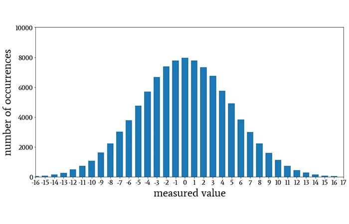
Normal Distribution If you measured the height of every single individual on the planet, or even a representative sample of them, the shape of that graph (often called “curve” in academic language) would be similar to this image:
This is the Normal Distribution (or Bell Curve), and it is the most important shape in risk management.12 It describes how randomness usually behaves. The very top of the hill represents the Mean (the average). This is what you “expect” to happen; in our stadium example, this is the average height (say, 5’9″). The vast majority of people will be average height, so their heights will be recorded as being clustered right around the middle.
If the Mean tells you where the peak is, Variance tells you how wide the hill is. It is a statistical measure showing how spread out a set of data points are from their average.13
Low Variance: Imagine a hill that looks like a needle. This means data points are tightly clustered. If you measured the height of 10,000 professional jockeys, the variance would be low—almost everyone is close to the average.14
High Variance: Imagine a hill that looks like a flattened pancake. This means data is widely spread out. If you measured the height of a random crowd containing jockeys and basketball players, the hill would be very wide.15
In risk management, mean tells you what usually happens; variance measures unpredictability and the potential for outcomes to be very different from the average, which is the essence of uncertainty.1617 A high variance means numbers are widely scattered, increasing the chance of both extreme positive and, crucially, extreme negative outcomes (losses).18 Low variance indicates they are clustered closely around the mean: it quantifies the dispersion or variability within a dataset.18 In the height data set, while most people would be average height, some people would be very short and others very tall as well. It’s just that the number of people who are not close to the average would fall off the farther away we get from the mean, or the middle of the bell curve.
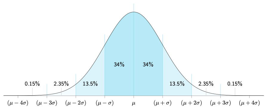
Normal Distribution divided into standard deviations distances from the mean.20
If Variance tells you the hill is “wide,” Standard Deviation (Sigma, or σ) tells you exactly how wide in real units. It is simply the square root of variance.
Think of Standard Deviation as the ruler for the Bell Curve.
1 Standard Deviation: In a normal distribution, about 68% of all outcomes happen within one standard deviation of the mean. If the average height is 5’9″ and the standard deviation is 3 inches, 68% of men are between 5’6″ and 6’0″.
2 Standard Deviations: Go out a bit further, and you capture 95% of all outcomes.
3 Standard Deviations: Go out three steps, and you capture 99.7% of everything.
In risk, when someone talks about a “Six Sigma” event (six standard deviations away from the average), they are talking about something so rare that it should theoretically almost never happen. And yet, in financial markets and complex systems, these “impossible” events happen surprisingly often.
Confidence2122 If a bank says, “We are 95% confident we won’t lose more than £1 million tomorrow,” they are essentially saying: “If tomorrow is a normal day (one of the 95%), we are safe. But if tomorrow is one of those rare, 1-in-20 bad days, all bets are off.”
In statistics, confidence is often explained using confidence intervals: at a 95% confidence level, the method used to build the interval would capture the true value about 95 times out of 100 repeated samples. That does not mean the true value has a 95% probability of being inside this specific interval; it means the procedure has 95% long-run reliability. This means, confidence intervals speak about frequency: how often do the unexpected or unwanted events happen. At 95%, they happen on any 5 days out of 100. at 99%, they happen once every 100 days.
For risk management, think of confidence levels as a dial for paranoia:
95% Confidence: You are planning for the normal bad days. You accept that on 1 day out of every 20 (roughly once a month), you will breach your limit.
99% Confidence: You are planning for the severe days. You only accept breaching your limit on 1 day out of 100 (roughly 2–3 times a year).
99.9% Confidence: You are planning for near-disaster. You only accept a breach once every 1,000 days (roughly once every 4 years).
The Micromort In the 1970s, Stanford professor Ronald Howard needed a way to compare diverse risks like skydiving, smoking, and driving. He invented the Micromort—a unit representing a one-in-a-million chance of death.23
This equalises different activities. Instead of vague fears (“is it safe to fly?”), we can use units:
1 Micromort is roughly the risk of driving 250 miles (400 km).24
1 Micromort is also the risk of flying 6,000 miles (9,600 km).24
NB: This post is now updated to include the 18th consecutive toss loss.
It’s come to my attention that we have lost the last 17 18 coin tosses in One Day International matches for men’s cricket,1 so here’s a continuation of our unfortunate probabilities.
Every coin toss is considered an independent event- the outcome of one fair coin toss will not have any impact on the outcomes of any other fair coin tosses.
The probability of two independent events happening at the same time is the product or multiplication of the probabilities of the two events in question. This is called “joint probability”, so If event A has probability P(A) and event B has probability P(B), and their outcomes do not affect each other, the probability that both occur is P(A) × P(B).
#
Date
Opponent
Venue
Captain
Toss Result
1
Nov 19, 2023
Australia
Ahmedabad
Rohit Sharma
Lost
2
Dec 17, 2023
South Africa
Centurion
KL Rahul
Lost
3
Dec 19, 2023
South Africa
Gqeberha
KL Rahul
Lost
4
Dec 21, 2023
South Africa
Paarl
KL Rahul
Lost
5
Feb 6, 2024
England
Hyderabad
Rohit Sharma
Lost
6
Feb 9, 2024
England
Visakhapatnam
Rohit Sharma
Lost
7
Feb 12, 2024
England
Rajkot
Rohit Sharma
Lost
8
Aug 10, 2024
Sri Lanka
Colombo
Rohit Sharma
Lost
9
Aug 12, 2024
Sri Lanka
Pallekele
Rohit Sharma
Lost
10
Aug 15, 2024
Sri Lanka
Dambulla
Rohit Sharma
Lost
11
Feb 20, 2025
Bangladesh
Dubai
Rohit Sharma
Lost
12
Feb 23, 2025
Pakistan
Dubai
Rohit Sharma
Lost
13
Mar 2, 2025
New Zealand
Dubai
Rohit Sharma
Lost
14
Mar 4, 2025
Australia
Dubai
Rohit Sharma
Lost
15
Mar 9, 2025
New Zealand
Dubai
Rohit Sharma
Lost
16
Oct 19, 2025
Australia
Perth
Shubman Gill
Lost
17
Oct 23, 2025
Australia
Adelaide
Shubman Gill
Lost
18
Oct 25, 2025
Australia
Sidney
Shubman Gill
Lost
India’s 17 18 consecutive ODI coin toss losses in men’s international cricket
You’ll notice that once again the tosses have been lost across tournaments, three different captains, and multiple venues (home and away), and the calling captains choosing heads or tails at random and India still losing every time.
Now, at first I thought that the all format streak of losing 16 consecutive tosses and this ODI streak of losing 17 consecutive tosses were just one series of unfortunate events, but now I want to understand what the probability is of these being considered separate streaks and both “events” still occurring.
So here are the two overlapping streaks:
The ODI-specific streak (Nov 2023–Oct 2025):17 18 consecutive ODI toss losses. Probability = (1/2)^17 = 1/131,072 ≈ 0.00076%(1/2)18 = 1/262,144 ≈ 0.000381%; and
The all-format streak (Jan–Oct 2025): 16 consecutive toss losses across formats. Probability = (1/2)16 = 1/65,536 ≈ 0.0015%.
And the probability that these two have coexisted is just the multiplication of the two independent streaks, which is P = (1/131072) × (1/262,144) = 1/8589934592, or about 1/8,600,000,000, which is one in 8.6 billion1/17179869184, or about 1/17,000,000,000, which is one in 17 billion.
As of mid-2025, the world population was estimated to be around 8.2 billion.2 So if in the middle of this year, if every single person had tossed a fair coin TWICE, there is a possibility that these two streaks would still not have overlapped. It’s an astronomical rarity, so of course we’re on the wrong side of it, *depressed emoji*.
In probability theory, there is a concept of waiting time. Waiting time in streak probability asks how long before you see the streak in question happen? So here it will ask, “How many tosses, on average, until you first see a streak of n consecutive heads (or losses, or wins)?” For a fair coin, the expected number of tosses (waiting time) to see an uninterrupted streak of length n is approximately: En = 2(n+1) – 2.3
In the formula, “n” is the length of the streak.
For a streak of 6 coin toss losses, we will have to wait for
E6 = 2(6+1) – 2
E6 = 27 – 2
E6 = 2 × 2 × 2 × 2 × 2 × 2 × 2 – 2
E6 = 128 – 2 = 126 coin tosses.
So, for our first streak of 16 consecutive coin toss losses, the world waited with bated breath for 217 – 2 = 131,070 fair tosses;
For the ODI 17 18 coin toss loss streak, we waited for 218 − 2 = 262,142 219 -2 = 524,286 fair tosses; and
For both to happen together, we waited 131,070 × 262,142524,286 fair tosses, or 68,718,166,020, or more than 34 68.7 billion fair coin tosses- A NUMBER SO WILD (okay, calm down, calm down) even cricket fans don’t expect it.
What the hell, my guys?
NB: I just realised that the most widely accepted scientific estimate for the age of the known universe is about 13.8 billion years,4 so the chances of these two streaks happening at all, let alone together, actually involves numbers several times greater than the entire age of the universe in years. Personal suggestion to Shubman Gill- havan karwale bhai.
India has now lost 16 consecutive coin tosses across all formats, with the streak extending from January 31, 2025, to October 2, 2025 (the West Indies – India Test match in Ahmedabad that concluded today). Here’s the baffling list by chronology:
Coin Toss Loss No.
Date
Match
Venue
Captain
1
Jan 31, 2025
4th T20I vs England
Pune
Suryakumar Yadav
2
Feb 02, 2025
5th T20I vs England
Mumbai (Wankhede)
Suryakumar Yadav
3
Feb 06, 2025
1st ODI vs England
Nagpur
Rohit Sharma
4
Feb 09, 2025
2nd ODI vs England
Cuttack
Rohit Sharma
5
Feb 12, 2025
3rd ODI vs England
Ahmedabad
Rohit Sharma
6
Feb 20, 2025
ODI vs Bangladesh
Dubai (Champions Trophy)
Rohit Sharma
7
Feb 23, 2025
ODI vs Pakistan
Dubai (Champions Trophy)
Rohit Sharma
8
Mar 02, 2025
ODI vs New Zealand
Dubai (Champions Trophy)
Rohit Sharma
9
Mar 04, 2025
ODI vs Australia
Dubai (Champions Trophy Semi-final)
Rohit Sharma
10
Mar 09, 2025
ODI vs New Zealand
Dubai (Champions Trophy Final)
Rohit Sharma
11
Jun 20, 2025
1st Test vs England
Leeds
Shubman Gill
12
Jul 02, 2025
2nd Test vs England
Birmingham
Shubman Gill
13
Jul 10, 2025
3rd Test vs England
Lord’s
Shubman Gill
14
Jul 23, 2025
4th Test vs England
Manchester
Shubman Gill
15
Jul 31, 2025
5th Test vs England
The Oval
Shubman Gill
16
Oct 02, 2025
1st Test vs West Indies
Ahmedabad
Shubman Gill
Indian Men’s toss losing streak
In mathematics, probability measures how likely an event is to occur, and it’s always expressed as a number between 0 (will never happen) and 1 (will definitely happen every time). For a standard fair coin toss, the probability of either heads or tails is exactly 0.5 (or 50%). This is because there are two possible and equally likely outcomes: the coin will either flip to heads or tails (not counting the vanishingly small number of times it may fall on its edge, in which case the toss will be repeated until a result is achieved anyway).
Every toss is also independent, which means that the result of one toss will have no impact on the result of any other toss. When events are independent, the probability of several events occurring in succession is the product (multiplication) of their individual probabilities. So, the probability of losing (or winning) two fair tosses in a row is: Probability of 2 losses = 0.5 × 0.5 = 0.25.
The probability of losing (or winning) 3 fair tosses in a row is therefore = 0.5 × 0.5 × 0.5, which is 0.125.
We’ve lost 16 consecutive tosses across formats, geographies, and captains. The probability of winning or losing a fair coin toss is 0.5 or 1/2. Which means the probability of losing 16 consecutive fair coin tosses is… (0.5)16, which equals 1 in 65,536, or ≈0.0000152588%.
Now, it really must be noted that a cricket coin toss is quite different from a simple game of coin toss between two people (though the mathematics remains exactly the same). The Indian skippers were not always the ones tossing the coin, neither were they always the ones calling heads or tails. In cricket, the standard procedure is that the host captain tosses while the visiting captain calls. However, at neutral venues where neither captain is the host, the procedure varies: a neutral party such as a match official or invited dignitary may toss the coin, or one of the captains may be chosen to toss, or tournament regulations may specify the exact protocol. This means India’s losing streak has transcended not just different formats, captains and venues, but also different toss procedures, making it an even weirder demonstration of statistical randomness.
I decided to investigate the mathematics of this absurdity.
0.0000152588% How rare is a 0.0000152588% chance of any event happening? Well, more people are struck by lightning annually,1 but fewer people are likely to die by meteorite strike2.
Similar things have happened in cricket before- The Netherlands have previously lost 11 consecutive tosses, and and several teams have lost 9 in a row.3 Rohit Sharma himself has lost 12 consecutively (equalling Brian Lara).3
Independence and the Gambler’s Fallacy The Gambler’s Fallacy is the (mistaken) belief that because India “lost so many times in a row,” they’re “due” for a win, but since each coin toss is independent and past outcomes have absolutely no impact on the next. Each toss remains a 50-50 chance, regardless of what’s happened before.
The Law of Large Numbers and the Nature of Streaks The Law of Large Numbers states that if an independent act is performed enough times, the outcomes of this independent event (the coin toss in our case) will eventually (that is, in the long term, given a large number of coin tosses) match the predicted probable outcome of that event (that is, 50% of the times the coin will flip heads, and 50% of the times it will flip tails), but this will of course include every coin toss ever, and not restrict itself to India’s male cricket captains.
This simply means that though the average outcome will even out to about 50% wins and losses, streaks such as 16 losses in a row are still possible, just extremely unlikely. Given enough cricket matches played, even “impossible” events are destined to surface from time to time. Cricket tosses represent a relatively small sample size in the grand scheme of probability. Even if we consider all international cricket matches ever played, this would still represent a small enough sample size where unusual streaks can and will occur (to understand this, compare every cricket toss to every coin toss that has ever happened in history).
Information Theory In Information Theory, the rarer an event is considered, the more surprising it is found to be. This means losing one toss is not surprising since there is a 50% chance of losing any one random fair toss. However, losing 16 tosses in a row must be considered very surprising because it involves the following outcomes:
Lose the first toss (50% probability), then lose the second toss (50% probability), then lose the third toss (50% probability), then lose the fourth toss (50% probability), then lose the fifth toss (50% probability)… then finally lose the 16th toss, also with a fifty percent probability that you could win it or lose it.
Which means that if nothing else, at least my bewilderment at the streak is justified.