Risk – III: Pricing Risk

A 40-year-old non-smoker in Delhi faces a measurable probability of dying in the next year. If the 40 year old is a woman, she will have a slightly better chance at life than a male counterpart. If she lives in a wealthy area, her chances are once again better than another woman living in a less privileged location.123

How do we know this? We know this because actuaries work with mortality and health data from millions of people, and build tables that segment risk by age, gender, smoking status, income, and even geography, to price policies accurately.4

Types of risk
Over time, experts have classified risk into different types. Here’s a table about the different types of risk:

RISK TYPEDEFINITIONCHARACTERISTICSEXAMPLES
HAZARD RISK (Pure Risk)56The possibility of loss from natural events or accidents. The oldest, most intuitive kind of risk.• Unintended—nobody wants them
• Objective frequency data—insurers have centuries of records
• Insurable—probability and consequence can be estimated from historical data
• Cannot create profit—only causes loss
• Fire and property damage
• Windstorms and hail
• Theft and burglary
• Flooding
• Liability from personal injury
OPERATIONAL RISK78910The risk that your business’s internal machinery breaks down. Unlike hazard risk, it’s inherent to doing business—you can’t eliminate it, only manage it. Also cannot be diversified away. Defined by Basel II as: “Risk of loss from inadequate or failed internal processes, people and systems, or external events.”• Inherent to operations—impossible to eliminate
• Non-diversifiable—all firms in an industry face similar operational risks
• Hard to quantify—driven by control quality and governance, which are difficult to measure
• Multiple sources—spans people, processes, systems, and external events
Process Failures: Accountant enters data incorrectly, leading to wrong financial statements; Wrong calculation of tax liabilities

Human Error: Surgeon operates on wrong patient; Employee sends confidential email to wrong recipient; Trader executes wrong order

System Failures: Bank’s payment system crashes; Company’s website goes down during peak shopping season; Database corruption losing customer data

Fraud: Employee embezzles funds; Vendor submits fake invoices; Internal collusion to bypass controls

External Events: Natural disaster destroys office; Key supplier suddenly defaults; Cyberattack from external actor
FINANCIAL RISK111213Risk from changes in financial variables: credit defaults, price movements, or inability to access funds. Encompasses three subcategories.• Market-driven—determined by supply and demand in public markets
• Observable prices—interest rates, bond spreads, stock prices are public
• High correlation—multiple financial risks often move together during crises
Credit Risk: Borrower fails to repay loan; Bank faces default

Market Risk (Interest Rate, Equity, Currency, Commodity): Interest rates rise, bond portfolio value falls; Stock prices decline; Rupee weakens against dollar; Oil prices spike increasing business costs

Liquidity Risk (Asset & Funding): Cannot sell asset when needed (asset liquidity); Cannot raise cash when obligations due (funding liquidity)
STRATEGIC RISK14Risk that your business strategy is wrong. Risk from strategic decisions and competitive threats that can derail long-term objectives. Highest impact, but low frequency.• High impact, low frequency—rare but potentially catastrophic
• Long-term consequences—effects persist for years
• Cross-functional impact—affects entire organization
• Forward-looking—requires anticipating future changes
• Not quantifiable—each situation is somewhat unique
Poor Strategy Decisions: Entering unviable new markets; Expanding too quickly into new industries; Pricing strategy that’s unprofitable

Competitive Threats: New disruptive competitor; Competitor’s aggressive pricing; Merger of competitors

Technological Disruption: Emerging technology makes business model obsolete (e.g., ride-sharing disrupting taxis); Failed innovation or delayed product launches

Resource Misalignment: Allocating resources to declining products instead of growth opportunities

Market/Industry Changes: Shift in customer needs and expectations; Regulatory changes forcing business model changes
COMPLIANCE & REGULATORY RISK15The risk that you violate laws, regulations, or internal policies, resulting in fines, legal action, or reputational damage. The regulatory environment is constantly changing.• Pervasive—affects all areas of organization
• Constantly evolving—new regulations, changing requirements
• Penalties escalating—fines and enforcement becoming more severe
• Jurisdiction-dependent—different rules in different countries
• Partly controllable—you can strengthen controls, but regulatory changes are external
Financial Crimes: Money laundering violations; Bribery and corruption; Sanctions violations

Data & Privacy: GDPR violations (Europe); CCPA violations (California); HIPAA violations (healthcare); Customer data breaches

Contract & Market Conduct: False advertising; Market manipulation; Insider trading; Misleading disclosures

Employment & Safety: Labor law violations; Health and safety violations; Harassment and discrimination

Industry-Specific: Healthcare regulations (HIPAA); Financial regulations (Banking Acts); Environmental regulations
REPUTATIONAL RISK1617The risk that negative publicity damages your brand, eroding customer trust, investor confidence, investor perception, or ability to attract talent. One of the hardest risks to quantify.• Hidden until it happens—not visible in normal operations
• Disproportionate impact—market values reputation more than the direct financial loss
• Self-inflicted worse than external—fraud damages reputation 2x more than accidents
• Long recovery time—trust takes years to rebuild
• Interconnected—affects customer base, employees, investors, partners simultaneously
Product/Service Failures: Volkswagen emissions scandal (2015): $30B+ in losses, brand destroyed, took years to recover; Boeing 737 MAX crashes: customer confidence shattered; Product recalls damaging trust

Ethical/Fraud Issues: Wells Fargo account scandal: reputation destroyed despite being largest bank; Facebook/Meta privacy scandals: customer trust eroded

Workplace Issues: Harassment scandals; Discrimination claims; Executive misconduct

Environmental/Social: Oil spills; Labor exploitation; Pollution incidents
CYBER & TECHNOLOGY RISK1819The risk of losses from disruption or failure of IT systems, data breaches, ransomware attacks, or technology obsolescence. Increasingly distinct from general operational risk.• Rapidly evolving threat landscape—new attack vectors constantly emerge
• Control-dependent—pricing based on current security posture, not history
• Insurance available—unlike most strategic risks, cyber can be insured
• Industry-dependent—high-risk sectors (finance, healthcare) pay more
• Improving controls reduce premiums—strong incentive alignment
Data Breaches: Hackers steal customer information; Personal data of millions exposed; Regulatory fines and lawsuits follow

Ransomware Attacks: Criminals lock you out of systems; Demand payment to restore access; Business operations halt

System Failures: Software bugs or aging infrastructure cause crashes; Website goes down; Payment systems fail

DDoS Attacks: Website flooded with traffic, becomes inaccessible; Business loses revenue during attack

Insider Threats: Disgruntled employee steals data; System administrator sabotages operations; Contractor misuses access
Different types of risks

Each of these types of risks attracts different prices. Here’s another table:

RISK TYPEDEFINITIONPRICING CHALLENGEKEY INSIGHT
HAZARD RISK (Pure Risk)56The possibility of loss from natural events or accidents. The oldest, most intuitive kind of risk.Relatively straightforward to price because: Historical data is abundant and reliable Frequency and severity are stable over timeEasiest to price. Insurers have vast datasets spanning centuries showing how often fires, floods, and accidents occur. This precision makes hazard risk the most competitively priced and cheapest form of risk insurance.
OPERATIONAL RISK78910The risk that your business’s internal machinery breaks down. Unlike hazard risk, it’s inherent to doing business—you can’t eliminate it, only manage it. Also cannot be diversified away. Defined by Basel II as: “Risk of loss from inadequate or failed internal processes, people and systems, or external events.”• Real drivers (control quality, governance, employee skill) are hard to measure
• Cannot use simple historical formulas
• Basel II uses crude proxy: operational risk capital = percentage of gross income
• Limited historical data compared to hazard risk
• Outcomes are correlated across firms during crises
Cannot diversify away. When 100 banks all face the same operational risk (say, a payment system cyberattack), they all suffer simultaneously. This systemic nature makes operational risk expensive to accept and pricing it requires judgment, not just formulas.
FINANCIAL RISK111213Risk from changes in financial variables: credit defaults, price movements, or inability to access funds. Encompasses three subcategories.• Models based on historical data miss tail risk (rare catastrophic events)
• Correlation assumptions break during crises (2008 showed this)
• Pricing assumes future resembles past
• Volatile and difficult to predict
Impossible to price accurately at extremes. Financial risk is driven by market sentiment, which can shift suddenly. Models work 99% of the time but fail catastrophically in the 1% (like 2008), when many risks materialize simultaneously.
STRATEGIC RISK14Risk that your business strategy is wrong. Risk from strategic decisions and competitive threats that can derail long-term objectives. Highest impact, but low frequency.• No historical data for “probability that our strategy fails”
• Each strategic decision is somewhat unique
• Cannot use formulas or actuarial tables
• Outcomes depend on management judgment and execution
• Extremely difficult to quantify in advance
Cannot be insured. Strategic risk is almost entirely uninsurable because each company’s strategy is unique. CEOs and boards must accept this risk as part of doing business. Pricing relies on scenario analysis and management judgment, not hard data.
COMPLIANCE & REGULATORY RISK15The risk that you violate laws, regulations, or internal policies, resulting in fines, legal action, or reputational damage. The regulatory environment is constantly changing.• Probability of enforcement depends on regulator priorities (which change)
• Penalties are often discretionary and unpredictable
• New regulations create retroactive compliance challenges
• Conflicting guidance from different regulators
• Costs increase with regulatory tightening
Costs are rising fast. Regulators are increasingly aggressive, penalties are larger, and reputational consequences are severe. Organizations must continuously invest in compliance infrastructure (legal teams, compliance officers, audits) as a cost of doing business.
REPUTATIONAL RISK1617The risk that negative publicity damages your brand, eroding customer trust, investor confidence, investor perception, or ability to attract talent. One of the hardest risks to quantify.• Stock price falls MORE than announced loss (2x for fraud, 1x for accidents)
• 26% of company value is directly attributable to reputation (one study)
• No standard pricing model
• Very difficult to quantify until it happens
• Historical data limited
Stock market values reputation more than we can measure. When a company announces a $1B fraud loss, stock price might fall 5% ($5B loss in value). The extra $4B is “reputational loss”—the market’s judgment that the company is now riskier. Yet most companies can’t quantify or insure this risk.
CYBER & TECHNOLOGY RISK1819The risk of losses from disruption or failure of IT systems, data breaches, ransomware attacks, or technology obsolescence. Increasingly distinct from general operational risk.• Unlike hazard risk (stable data over decades), cyber threats evolve rapidly
• Historical data is unreliable—new attack types didn’t exist 5 years ago
• Pricing focuses on current security posture not past incidents
• Rapidly changing insurance market (premiums spiked 80% in 2021-2022)
• Standardization emerging (ISO 27001, NIST)
Pricing is behavior-based. Unlike traditional insurance (fixed premium regardless of actions), cyber insurance prices based on your current controls. Companies with firewalls, multi-factor authentication, and ISO 27001 certification pay ₹80,000/year. Those with weak security might pay ₹3,00,000 or be denied coverage. This creates powerful incentives to improve security.
Pricing different types of risks

General principles of pricing risk
People react in different ways to risk. Some of us prefer the straight and narrow and others don’t think much of doing things that would be considered too risky by others- think of how some don’t mind skydiving, whereas others prefer their feet firmly on the ground. There are risks associated with both skydiving, and staying on the Earth, but different people like different things.

Therefore, risk can technically be transferred from one person to another. And this can be offered as a business service, for a price.

Now, before we go into this further, please understand that some risks can never be transferred- just that the effect of their impact can be mitigated. People will die, that is life. But by buying term insurance, we can ensure our families don’t suffer financial loss as well as the loss of our love and support. Similarly, living beings get sick- by purchasing health insurance we can just make sure we don’t face financial difficulties if we ourselves get sick in a way that costs a lot of money to fix. We are not transferring the death and decay, we are transferring the financial cost of these events.

1. The Formula2021
With that out of the way, when someone asks you to bear their risk, you charge them a price. That price is made up of several components:

Price of Risk = Expected Loss + Administrative Costs + Risk Loading + Profit Margin

Where:

  • Expected Loss is simply: Probability × Consequence. If there’s a 2% chance of a ₹100,000 loss, the expected loss is ₹2,000.
  • Administrative Costs are the cost of doing business. For an insurer, this includes underwriting (reviewing your application), policy servicing (managing your account), claims processing, and marketing. For a bank, it includes loan documentation, monitoring your creditworthiness, and collecting payments if you default.
  • Risk Loading is the “insurance premium on the insurance premium.” It’s an extra charge you demand to accept the fact that reality might differ from your expectations. This is where variance becomes critical.22
  • Profit Margin is what you keep as profit.

2. Variance

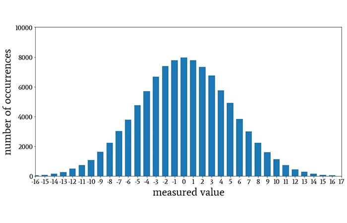
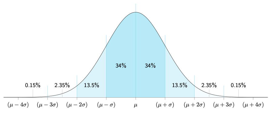
Variance is uncertainty about whether actual outcomes will match expected outcomes. As risk increases, variance often increases faster. Why? This happens because most people will fall closer to the middle of the normal distribution (discussed in the post linked at the beginning of the paragraph), but as risk increases, the number of people who are either that risky or are willing to take that risk are fewer and fewer (few will skydive, more will bungee jump, most will fly commercial). The fewer the number of people to whom a risk applies, greater the chances of variance (because the insurer has fewer people over whom to spread the risk). In other words, the law of large numbers works less effectively with small groups. With 1 million people, outcomes average out predictably, so let’s say you get the same or very similar number of claims every year. With 50 people, you might get zero claims one year and three claims the next—massive volatility.

I just want to be sure this is clear, so here is another example. Suppose two people pool their money every month, and decide that if one of them gets sick, the sick person can to use a certain percentage of the total money pooled (collected) by both of them to pay for the treatment. It is possible that for many years no one gets sick, but it is also possible that one (50%) of the total contributors or both (100% of the total contributors) get sick one day. On the other hand, in a pooled health insurance which has many contributors, say 1 million contributors, if 1 person gets sick, they are 1/1,000,000 of the total number of contributors (or 0.0001% of the pool- much, much less than 50%, right?).

Secondly, higher-risk individuals have more uncertain outcomes—meaning it’s harder to predict exactly what will happen. A skydiver faces multiple possible outcomes with varying probabilities: they could live unharmed, break bones, die from equipment failure, die from a heart attack mid-jump, or face other unpredictable complications. Each outcome has a different probability, making the overall risk calculation more complex. In contrast, a person simply walking on the ground faces far fewer potential causes of serious injury or death, so the range of possible outcomes (variance) is much narrower. Another way of looking at this is that a 30 year old healthy non smoker likely has fewer known causes of death historically than a 70 year old smoker.

This is why insurance premiums for risky people increase disproportionately:

  • The insurer must hold more capital to protect against bad luck.
  • A 30-year-old non-smoker with a 0.05% probability of death in a year might have a premium of ₹3,000.
  • A 60-year-old smoker with a 1% probability of death (20x higher) doesn’t pay 20x the premium (₹60,000). They pay 50x+ the premium (₹1,50,000 or more) because:
    • The absolute expected loss is 20x higher.
    • The variance around that expected loss is also much higher (more uncertainty about outcomes).

Insurers also worry about correlation—the risk that many claims happen simultaneously. A life insurer pricing individual deaths assumes they’re independent. But if a pandemic strikes, many policyholders might die at once. This correlation risk requires extra capital, adding to the risk loading.2324

Uncertainty
When an insurer lacks information about a particular risk, they will charge more for it, because they do not know how potent the risk is, or how frequently it occurs.2526

Suppose a bank is deciding whether to lend to two borrowers, both with self-reported income of ₹10 lakhs per year.

  • Borrower A: A salaried employee with 10 years of bank statements, tax returns, and employer verification. The bank has rich information about their actual, consistent income.
  • Borrower B: A self-employed consultant with only 2 years of tax returns. Income has varied between ₹5 lakhs and ₹15 lakhs per year. The bank’s uncertainty about their true ability to repay is high.

Both might have estimated default probabilities of, say, 2% based on available data. But the bank will charge Borrower B a higher interest rate, not because their actual default probability is higher, but because the bank’s uncertainty about that probability is higher.

This principle explains all of the following:

  • Businesses in developed countries with strong financial reporting get cheaper capital than those in developing countries with weak disclosure.2728
  • Companies listed on stock exchanges get better rates than private companies (more transparency).29
  • Established firms in regulated industries get better rates than startups in emerging sectors.30

Therefore, the more standardised and measurable a risk, the cheaper it is to price and the lower the price demanded. Insurance for hazard risk (with centuries of actuarial data) is cheaper relative to coverage than climate insurance (with only decades of data).31 VaR models for market risk are widely accepted because market prices are observable. But there’s no standard model for reputational risk, so it’s not widely insured.32

This creates a system where:

  • Predictable, measurable, insurable risks get priced accurately and competitively.
  • Unpredictable, hard-to-measure risks are either:
    • Not insured at all (like most strategic risk).
    • Priced with huge margins because of the uncertainty (like reputational risk).

This is a profound source of inefficiency in capital allocation. Risks that are easiest to measure and quantify get the cheapest pricing and most capital. Risks that are hardest to measure—sometimes the ones that matter most—get starved of capital or don’t get priced at all.

A problem that has emerged from this is that historical models can simply not price tail risks (risks at the corners of normal distributions). An area this affects is climate risk, and its pricing.3334 A different example many of us lived through was the 2008-09 subprime financial crisis. In 2008, banks had calculated that simultaneous mortgage defaults across their portfolio should happen once every few thousand years. Yet it happened in 2007-2008. Why?35

The models went with historical data and assumed:

  • Housing prices wouldn’t decline nationwide (they always went up historically).36
  • Unemployment wouldn’t spike across industries simultaneously.37
  • Banks wouldn’t stop lending to each other.37

But all three happened together, creating a “perfect storm” that the models had assigned nearly zero probability. The tail risk was real; the pricing was wrong. Financial institutions now conduct stress testing—asking, “What if housing prices fell 30%? What if unemployment doubled? What if credit markets froze?“—precisely because historical models miss these scenarios.

Thus, if a financial advisor saying “stocks haven’t crashed in 50 years, so the probability is very low” is engaging in tail risk underpricing, and yet, we do still use the method to price some kinds of risk. The next section talks about this and other methods of risk pricing.

Pricing different risks

Methodology 1: The Actuarial Approach (Hazard Risk)4
Insurance companies maintain vast databases of historical claims. For life insurance, they track millions of deaths by age, gender, health status, and lifestyle. For home insurance, they track fire and weather damage claims by location and property type. For auto insurance, they track accidents by driver age, vehicle type, and location. From this data, actuaries calculate frequency (how often does the event occur?) and severity (how much damage when it does?). The math relies on:

  1. Having huge sample sizes (law of large numbers).
  2. Accurate historical data (actuarial tables updated constantly).
  3. Stable risk—the probability of death doesn’t change dramatically over time.
  • Why this works: Hazard risk has all these properties. Insurers have massive datasets, deaths are well-documented, and the probability of death doesn’t swing wildly year to year.
  • Why it fails: When underlying assumptions break, actuarial models fail. During COVID-19, mortality rates spiked unexpectedly, and life insurers faced massive losses. The historical tables became temporarily unreliable.

Methodology 2: The Credit Approach (Financial Risk)383940
Banks estimate the Probability of Default (PD) of a borrower. This comes from:

  1. Credit ratings (developed from historical default rates of companies with similar characteristics).
  2. Credit scores (statistical models predicting default probability).
  3. Loan characteristics (collateral, loan-to-value ratio, term length).

They also estimate Loss Given Default (LGD)—how much money the bank recovers if the borrower defaults. If a borrower defaults on a ₹100 lakh loan backed by ₹60 lakhs of collateral, the LGD is 40%.

The interest rate spread (the premium above the risk-free rate) is then set approximately as:

Interest Rate = Risk-Free Rate + (PD × LGD + Risk Loading) + Liquidity Premium + Other Premiums41

Other premiums:

Risk PremiumExplanation
Credit Risk Premium42Compensation for the probability that the borrower defaults and the amount the lender loses if they do (PD × LGD)
Liquidity Premium43Compensation for holding an asset that is difficult to sell quickly (e.g., corporate loans are less liquid than government bonds)
Inflation Risk Premium44Compensation for uncertainty about future inflation; if inflation is higher than expected, the real value of repayments falls
Term Premium44Compensation for lending money for longer periods; longer loans have more uncertainty about interest rates and borrower circumstances
Currency Risk Premium45Compensation for the risk that exchange rates move unfavorably; relevant when borrowing in a foreign currency
Sovereign Risk Premium46Compensation for political and economic instability in the borrower’s country; reflects country-level risk beyond individual borrower risk
Regulatory Risk Premium47Compensation for the risk that changes in laws or regulations will harm the lender’s position
Prepayment Risk Premium48Compensation for the risk that the borrower repays early (often when interest rates fall), causing the lender to reinvest at lower rates
Concentration Risk Premium49Compensation for lending a large amount to a single borrower or sector, which increases the lender’s exposure
Call Risk Premium50Compensation for the risk that the bond issuer redeems the bond early, leaving investors with reinvestment risk
Event Risk Premium51Compensation for the risk of specific one-off events (mergers, leveraged buyouts, natural disasters) that suddenly change creditworthiness
Convertibility Risk Premium48Compensation for the risk that capital controls or currency restrictions prevent conversion to foreign currency
Transfer Risk Premium52Compensation for the risk that a government blocks or restricts cross-border payments, even if the borrower wants to pay
Different types of risk premiums that may be charged by banks on loans
  • Why this works: Credit markets are large and competitive. Banks have decades of default data. Collateral can be valued. PD and LGD can be estimated with reasonable accuracy.
  • Why it fails: When credit conditions change suddenly (as in 2008), the relationship between PD and actual defaults breaks. A borrower who seemed safe (PD 1%) might suddenly have a 20% probability of default if the economy collapses. This is called “correlation risk”—risks that seemed independent are actually correlated, and they all materialize simultaneously.

Methodology 3: Value at Risk (Market Risk)5354
When investment banks, traders, and portfolio managers hold stocks, bonds, or other financial assets, they face a fundamental question: “How much could we lose on a bad day?” Value at Risk (VaR) answers this question: “What’s the maximum loss I might suffer with 95% confidence over a given time period (usually one day)?”

Suppose you hold a portfolio of Indian stocks worth ₹1 crore. You want to know your VaR at 95% confidence for one day.

Here’s how you calculate it:

  1. Gather historical data: Look at how much your portfolio’s value changed each day over the past 5 years (roughly 1,250 trading days).
  2. Calculate daily returns: On some days, your portfolio gained 2%. On others, it lost 3%. Most days, changes were small (±0.5%).
  3. Rank all the losses: Sort all the daily changes from worst to best.
    • Worst day: -10% (₹10 lakh loss)
    • 95% of days: losses were less than -7%
    • Typical days: ±1%
  4. Identify the 95th percentile: Find the loss that was exceeded on only 5% of days (the worst 5% of outcomes). Let’s say this was -7%.

Your VaR is ₹7 lakhs.

What this means in plain English:
“Based on historical patterns, we are 95% confident that on any given day, we won’t lose more than ₹7 lakhs. But on 1 out of every 20 days (5% of the time), we might lose more than this—possibly much more.”

How Banks Use VaR:

Banks use VaR for three main purposes:

  1. Setting risk limits: “No trader can hold a position with VaR greater than ₹50 lakhs.”
  2. Allocating capital: “This trading desk’s portfolio has VaR of ₹2 crore, so we must set aside ₹2 crore in capital to cover potential losses.”
  3. Pricing risk: “We need to earn at least 10% return on our ₹2 crore capital (₹20 lakhs per year), so the portfolio must generate returns higher than the risk-free rate by at least this amount.”
  • Why this works: Market prices are observable and historical data is abundant. VaR is simple to calculate and widely understood.
  • Why it fails spectacularly: VaR assumes the future resembles the past. When it doesn’t—when a “tail risk” event occurs that’s much worse than historical data suggested—VaR provides false confidence. Black swan events—outliers far beyond historical norms—happen more often in real markets than VaR predicts. This is why sophisticated risk managers now conduct stress tests: “What if housing fell 30%? What if correlation across assets went to 1.0 (everything moves together)?” These scenarios often have probabilities that can’t be estimated from historical data.

Methodology 4: Reputational Risk Quantification16175556
Reputational risk is one of the hardest to price because reputation damage is:

  • Invisible until it happens
  • Subjective (how much is brand trust worth?)
  • Interconnected (affects customers, employees, investors, suppliers simultaneously)

Yet we know reputation has enormous value because research shows that roughly 26% of a company’s market value is directly attributable to its reputation.57 So how do we price something intangible?

The Stock Price Method: When a company announces a major negative event (fraud, scandal, product failure), the stock price falls. But often, the stock price falls more than the announced financial loss. The difference is the market’s estimate of reputational damage.

Reputation Risk Quantification Models that try to systematically price reputation risk:

  1. Identify reputation threats: Product recalls, scandals, poor earnings, social media backlash
  2. Estimate frequency: How often does each type of event happen in this industry?
  3. Model financial impact: Customer loss, revenue decline, employee turnover costs
  4. Quantify total effect: Project impact on profits over 3-5 years

However, unlike life insurance (centuries of death data) or credit risk (decades of default data), reputation damage is:

  • Context-dependent: The same scandal might destroy one company but barely hurt another
  • Hard to predict: Social media can amplify or diminish reputational harm unpredictably
  • Self-reinforcing: Initial reputation damage can trigger customer flight, making things worse

This is why most companies don’t buy reputation risk insurance:

  • Insurers can’t agree on how to price it
  • Coverage is extremely expensive when available
  • Policies have many exclusions

So reputation risk remains largely self-insured—companies must manage it through strong governance, ethical culture, and crisis response planning, but they can’t transfer it to an insurer the way they can with fire risk or credit risk.

Methodology 5: The Security Audit Approach (Cyber Risk)585960
Historically treated as operational risk, cyber risk is now often priced separately. Unlike traditional hazard risk (based on decades of historical data), cyber insurance prices risk based on current security posture. Insurers conduct security audits assessing:

  • Business context: Industry (finance = higher risk), revenue size, number of employees, data sensitivity.
  • Technical controls: Firewalls, intrusion detection, endpoint protection, multi-factor authentication.
  • Process maturity: Patch management, vulnerability assessment, incident response plans.
  • Compliance: Certifications like ISO 27001 or NIST Cybersecurity Framework.
  • Training: Employee security awareness, phishing simulations.

Unlike traditional insurance (where you pay a fixed premium regardless of your actions), cyber insurance creates incentive alignment. Companies are rewarded for improving security. This is why cyber premiums vary so widely—from ₹80,000 to ₹3,00,000 for similar coverage, depending on security posture, so if the insured company becomes better prepared, its insurance premium can go down. The industry is evolving rapidly. As cyber threats evolve, pricing models are updated. Premiums spiked 80% in 2021-2022 (due to ransomware explosion) but have stabilized as companies improved controls and insurers refined models.

Methodology 6: Scenario Analysis (Strategic Risk)6162
Strategic risk is fundamentally different because:

  • Can’t be insured—no insurer will cover “your strategy might be wrong”
  • No historical data exists for “probability our specific strategy fails”
  • Each decision is unique—your market entry isn’t comparable to another company’s
  • Outcomes depend on management judgment, execution capability, and competitor actions

Instead of formulas, companies use scenario analysis—imagining multiple possible futures and testing strategy robustness across them.

The Process:

Step 1: Define the Current Strategy: Example: An e-commerce company currently selling books and electronics is considering expanding into furniture delivery.

Step 2: Imagine Alternative Futures (Scenarios): Scenario planning typically develops 3-5 scenarios representing different ways the future might unfold. Assign probabilities to different scenarios and how much loss your company would bear, for example, a company may have a scenario that

Step 3: Calculate Expected Value (With Huge Caveats).

Example:

Scenario A: “Competitive Onslaught”

  • 3 major competitors enter within 18 months
  • Price war erupts, margins drop 20%
  • Company loses ₹50 crore over 3 years
  • Probability: 60%

Scenario B: “Logistics Nightmare”

  • Delivery complexity exceeds expectations
  • High return rates (15%)
  • Company loses ₹30 crore
  • Probability: 40%

Scenario C: “Weak Demand”

  • Market adoption slower than projected
  • Company loses ₹80 crore
  • Probability: 30%

Scenario D: “Success”

  • Market responds positively
  • Company gains ₹150 crore
  • Probability: 20%

Note: Probabilities don’t need to sum to 100% because scenarios aren’t mutually exclusive—multiple scenarios could occur simultaneously (e.g., you could face both competitive pressure AND logistics challenges).

Expected Outcome = (Probability of Scenario × Impact)

= (0.6 × -₹50cr) + (0.4 × -₹30cr) + (0.3 × -₹80cr) + (0.2 × +₹150cr)
= -₹30cr – ₹12cr – ₹24cr + ₹30cr
-₹36 crore expected loss

  • Why this works: Strategic risk isn’t insurable. There’s no historical data on “furniture market entry outcomes” for this specific company. Each strategic decision is somewhat unique. Organizations can’t buy insurance for strategic risk; they must manage it through planning, contingency analysis, and management judgment.
  • Why it fails: Scenarios often miss the most important surprises. In 2020, COVID-19 wasn’t in most companies’ scenarios. When reality diverges from scenarios, organizations must adapt on the fly. This is why CEOs, not risk managers, bear ultimate responsibility for strategic risk.

Sources

  1. Life Actuarial (A) Task Force – APF CSO VM-M (2015)
  2. Gender and Smoker Distinct Mortality Table Development – Ghosh & Krishnaswamy
  3. Socioeconomic inequality in life expectancy in India – BMJ Global Health
  4. Big Data and the Future Actuary – Society of Actuaries
  5. What Is Pure Risk? – Investopedia
  6. Types of Risks—Risk Exposures – FlatWorld (Baranoff)
  7. Operational Risk – Supervisory Guidelines for the AMA – BIS (BCBS196)
  8. Module 3 – Operational Risk Guidance – GFSC
  9. Operational Risk – Basel 3.1 Implementation – Bank of England
  10. Operational Risk Management: The Ultimate Guide – MetricStream
  11. Credit risk, market risk, operational risk and liquidity risk – IndianEconomy.com
  12. Types of Financial Risks – Fiveable
  13. Categories of Risk – OCC
  14. Categories of Risk – OCC (duplicate link)
  15. Operational Risk Management: The Ultimate Guide – MetricStream (duplicate link)
  16. The Market Reaction to Operational Loss Announcements – Boston Fed
  17. Reputational Risk – Does it really Matter Against Financial Risk? – GARP
  18. Cyber Insurance in India – DSCI
  19. Reality check on the future of the cyber insurance market – Swiss Re
  20. Expense Load – IRMI
  21. Chapter 7 – Premium Foundations – Loss Data Analytics (open text)
  22. The Theory of Insurance Risk Premiums – Kahane (ASTIN / CAS)
  23. A review of capital requirements for pandemic risk – BIS FSI Briefs
  24. An alternative approach to manage mortality catastrophe risks under Solvency II
  25. Recursive correlation between voluntary disclosure, cost of capital, and firm value
  26. Cost of capital and earnings transparency – ScienceDirect
  27. Disclosure and cost of equity capital in emerging markets – ScienceDirect
  28. Effect of integrated reporting quality disclosure on cost of equity capital
  29. Going rate: How the cost of debt differs for private and public firms – Notre Dame
  30. Rate of Return Regulation Revisited (utilities) – Haas Berkeley working paper
  31. Climate Change Risk Assessment for the Insurance Industry – Geneva Association
  32. Assessing the Risks of Insuring Reputation Risk – Actuaries / CRO Forum
  33. Tailoring tail risk models for clean energy investments – Nature HSS Communications
  34. Climate Change Risk Assessment for the Insurance Industry – Geneva Association (duplicate link)
  35. Incorrectly Applying Default Correlation Theory: Causes of the Subprime Mortgage Crisis – NHSJS
  36. The Central Role of Home Prices in the Current Financial Crisis – Brookings
  37. Risk Management Lessons from the Global Banking Crisis – SEC / FSB
  38. Expected Loss (EL): Definition, Calculation, and Importance – CFI
  39. Loss Given Default (LGD) – Wall Street Prep
  40. Banking Risk Management (PD, EAD, LGD) – Roopya
  41. An Empirical Decomposition of Risk and Liquidity in Nominal and Inflation‑Indexed Yields – NBER
  42. The Hidden Risks of Private Credit – and How to Spot Them – GARP
  43. What Is Risk Premia – GreenCo ESG
  44. Interest Rate as the Sum of Real Risk‑free Rate and Risk Premiums – AnalystPrep
  45. Categories of Risk – OCC (duplicate link)
  46. Decomposing Government Yield Spreads into Credit and Liquidity Components – Danmarks Nationalbank
  47. Cost of Capital and Capital Markets: A Primer for Utility Regulators – NARUC
  48. Portfolio Risk Management & Investment – ETDB
  49. Concentration Risk on the Buy Side of Credit Markets – CFA Institute Blog
  50. Climate change financial risks: Implications for asset pricing and risk management – ScienceDirect
  51. Event Risk Premia – Sebastian Stoeckl (slides)
  52. Transfer of Risk – Investopedia
  53. Value at Risk (VaR) Models – QuestDB
  54. Introduction to Value at Risk (VaR) – QuantInsti
  55. Reputational Risk Quantification Model – WTW
  56. Reputational risk – the elephant in the room – Airmic
  57. $13.8 TRILLION IN PLAIN SIGHT – The Reputation Driving S&P 500 Value – Echo Research
  58. Cybersecurity Insurance Audit – Insureon
  59. Preparing for Cyber Insurance Audits with Compliance Scanners – ConnectSecure
  60. How to Reduce your Cyber Liability Insurance Premium – Databrackets
  61. Scenario Analysis Explained – Investopedia
  62. Scenario Analysis: Definition, Process, and Benefits – NetSuite

GHG Accounting: ISO 14064-1

Note: I know this is quite technical, but it’s about accounting, so that’s natural. Financial accounting tends to be technical too, right?

The ISO 14064 series is a family of international standards by the International Organization for Standardization (ISO) for quantification, monitoring, reporting, and verification of GHG emissions. They were developed by Technical Committee ISO/TC 207 on Environmental Management, Subcommittee SC 7 on Greenhouse Gas Management, can be adopted across different sectors, regions, and organisational types.

The ISO 14064 series currently comprises four main parts:

  • ISO 14064-1:2018 – “Greenhouse gases – Part 1: Specification with guidance at the organisation level for quantification and reporting of greenhouse gas emissions and removals.” This standard enables organisations to measure and report their total greenhouse gas emissions and removals.
  • ISO 14064-2:2019 – “Greenhouse gases – Part 2: Specification with guidance at the project level for quantification, monitoring and reporting of greenhouse gas emission reductions or removal enhancements.” This standard applies to specific projects designed to reduce emissions or enhance carbon removals, such as renewable energy installations, energy efficiency retrofits, reforestation programs, or methane capture projects.
  • ISO 14064-3:2019 – “Greenhouse gases – Part 3: Specification with guidance for the verification and validation of greenhouse gas statements.” This standard provides the framework for independent third-party verification and validation of GHG claims. It is the assurance mechanism that gives stakeholders confidence in reported emissions data.
  • ISO/TS 14064-4:2025 – “Greenhouse gases – Part 4: Guidance for the application of ISO 14064-1.” This newest addition, published in November 2025, is a Technical Specification that provides practical, step-by-step guidance for implementing ISO 14064-1. It bridges the gap between the normative requirements of the standard and real-world application, with detailed examples and case studies for different organisational types and sectors.

Additionally, the broader ISO 14060 family includes ISO 14065:2020 (requirements for bodies validating and verifying GHG statements), ISO 14066:2023 (competence requirements for verifiers and validators), and ISO 14067:2018 (carbon footprint of products).

This ecosystem of standards creates a framework:

  1. Organisations use ISO 14064-1 and 14064-4 to calculate their emissions;
  2. Project developers use ISO 14064-2 to quantify project benefits;
  3. Independent verifiers use ISO 14064-3 to audit these claims; and a
  4. Accreditation bodies use ISO 14065 and 14066 to ensure the competence and impartiality of the verifiers themselves.

The Five Core Principles

  1. Relevance: Select the GHG sources, GHG sinks, GHG reservoirs, data and methodologies appropriate to the needs of the intended user.
  2. Completeness: Include all relevant GHG emissions and removals.
  3. Consistency: Enable meaningful comparisons in GHG-related information.
  4. Accuracy: Reduce bias and uncertainties as far as is practical.
  5. Transparency: Disclose sufficient and appropriate GHG-related information to allow intended users to make decisions with reasonable confidence.

As stated explicitly in ISO 14064-1, “The application of principles is fundamental to ensure that GHG-related information is a true and fair account. The principles are the basis for, and will guide the application of, the requirements in this document”.

Relevance: Appropriateness to User Needs
This principle recognises that GHG inventories and reports serve specific purposes and must be designed to meet the needs of those who will rely on the information to make decisions.

Relevance begins with clearly identifying the intended users of the GHG inventory and understanding their information needs. Intended users may include the organisation’s own management, investors, lenders, customers, regulators, GHG programme administrators, or other stakeholders. Different users may have different information needs. For example, investors may focus primarily on climate-related financial risks and opportunities, while regulators may require specific emissions data for compliance purposes.

The relevance principle requires organisations to make appropriate boundary decisions (determining which operations, facilities, and emissions sources to include in the inventory based on what is material and meaningful to intended users): an inventory that excludes significant emission sources or includes irrelevant information fails to serve user needs effectively.

In practice, applying the relevance principle means that organisations must engage with their stakeholders to understand what information they need and why, design inventory boundaries and methodologies to provide this information, focus effort on quantifying the most significant emissions sources, and regularly reassess whether the inventory continues to meet user needs as circumstances change.

Completeness: Including All Relevant Emissions
The completeness principle requires organisations to include all relevant GHG emissions and removals within the chosen inventory boundaries. This principle ensures that GHG inventories provide a comprehensive picture of an organisation’s climate impact rather than selectively reporting only favorable information.

Completeness operates at multiple levels. At the broadest level, it requires that organisations establish appropriate organisational and reporting boundaries and then include all sources and sinks within those boundaries. For organisational-level inventories under ISO 14064-1, this means accounting for all facilities and operations that fall within the defined organisational boundary, whether based on control or equity share. It also means including both direct emissions from sources owned or controlled by the organisation and indirect emissions that are consequences of organisational activities.

The 2018 revision fundamentally changed how organizations handle indirect emissions. Instead of treating “Scope 3” as a monolithic category, ISO now requires systematic evaluation across six specific categories. This shift reflects reality: a manufacturer’s supply chain emissions (Category 4) and product use-phase emissions (Category 5) are fundamentally different and require different strategies. Organisations must systematically identify potential sources of indirect emissions throughout their value chains and include those that are determined to be significant based on magnitude, influence, risk, and stakeholder concerns. The real problem here is data availability: an organisation might know its own production emissions precisely, but will struggle to get Scope 3 data from thousands of distributors, and this makes implementation messy and imprecise.

An important aspect of completeness is the treatment of exclusions. If specific emissions sources or greenhouse gases are excluded from the inventory, ISO 14064-1 requires organisations to disclose and justify these exclusions. Justifications must be based on legitimate reasons such as immateriality, lack of influence, or technical measurement challenges, not simply on a desire to report lower emissions.

For GHG projects under ISO 14064-2, completeness requires identifying and quantifying emissions and removals from all relevant sources, sinks, and reservoirs affected by the project, including controlled, related, and affected SSRs. Failure to account for emission increases from affected sources (often called leakage) would result in overstatement of project benefits.

Consistency: Enabling Meaningful Comparisons
The consistency principle requires that organisations enable meaningful comparisons in GHG-related information over time and, where relevant, across organisations. Consistency is essential for tracking progress toward emission reduction targets, assessing the effectiveness of mitigation initiatives, and enabling external stakeholders to compare performance across organisations or sectors.

Consistency has several dimensions. It requires using consistent methodologies, boundaries, and assumptions over time when quantifying and reporting emissions. When an organisation measures its emissions in one year using specific methodologies and emission factors, it should apply the same approaches in subsequent years to enable valid comparisons.

It is important to note that consistency does not mean organisations can never improve their methodologies or expand their boundaries. Organisations may and should refine their approaches over time to improve accuracy, expand scope, or respond to changing circumstances. However, when such changes occur, consistency requires transparent documentation of what changed and why, recalculation of prior years where necessary to maintain comparability, and clear explanation in reports so users understand the nature and impact of changes.

Case in point, the base year concept embodied in ISO 14064-1 is central to applying the consistency principle. Organisations select a specific historical period as their base year against which future emissions are compared. The base year serves as the reference point for measuring progress toward reduction targets. ISO 14064-1 requires organisations to establish policies for recalculating base year emissions when significant changes occur to organisational structure, boundaries, methodologies, or discovered errors. These recalculation policies ensure that year-over-year comparisons remain valid even as organisations evolve.

The recalculation policy is most commonly triggered by three types of organisational change. First, structural changes: acquisitions, divestitures, or mergers that materially alter the scope of operations. ISO 14064-1 and the GHG Protocol typically define “material” as changes exceeding 5% of Scope 1 and Scope 2 emissions in the base year. For example, if a retail company acquires a logistics provider representing an additional 6% of historical emissions, the base year must be recalculated to include that logistics provider, enabling fair year-on-year comparison. Second, methodology improvements: when an organisation discovers better data or more appropriate emission factors. If a facility previously used regional electricity emission factors but gains access to grid-specific data, or if a company previously estimated employee commuting emissions using averages but now collects actual commute data, these improvements warrant recalculation. The driver is not change for its own sake, but the principle that prior years should benefit from improved accuracy just as current years do. Third, discovered errors: when an organisation identifies that prior-year calculations were systematically wrong—either over or understating emissions—recalculation is not optional; it is mandatory. Transparency requires disclosing both the error and its magnitude, then correcting the historical record. Organisations often establish a threshold (commonly 5%) below which minor corrections do not trigger full recalculation; instead, they are noted as adjustments in the current year. 

Accuracy: Reducing Bias and Uncertainty
Accuracy involves reducing systematic bias and reducing uncertainty.

  • Systematic bias occurs when quantification methods consistently overstate or understate actual emissions. For example, using an emission factor that is inappropriately high or low for the specific activity being quantified would introduce bias. The accuracy principle requires ensuring that quantification approaches are systematically neither over nor under actual emissions, as far as can be judged.
  • Uncertainty refers to the range of possible values that could be reasonably attributed to a quantified amount. All emission estimates involve some degree of uncertainty arising from measurement imprecision, estimation methods, sampling approaches, lack of complete data, or natural variability. The accuracy principle requires reducing these uncertainties as far as is practical through using high-quality data, appropriate methodologies, and robust measurement and calculation procedures. ISO 14064-1 requires organisations to assess uncertainty in their GHG inventories, providing both quantitative estimates of the likely range of values and qualitative descriptions of the causes of uncertainty. This assessment helps organisations identify where improvements in data quality or methodology could most effectively reduce overall inventory uncertainty.

Achieving accuracy begins with selecting appropriate quantification approaches. ISO 14064-1 recognises multiple approaches to quantification, including direct measurement of emissions, mass balance calculations, and activity-based calculations using emission factors. The most accurate approach depends on the specific source, data availability, and the significance of the emission source.

Organisations should also prioritise primary data (data obtained from direct measurement or calculation based on direct measurements) over secondary data from generic databases. Site-specific data obtained within the organisational boundary is preferable to industry-average or regional data. However, the accuracy principle also recognises practical constraints—perfect accuracy is often unachievable and unnecessary, particularly for minor emission sources.

The requirement to separately report biogenic CO₂ from fossil fuel CO₂ in Category 1 may seem like a technical distinction, but it reflects a fundamental policy divergence emerging globally. Biogenic emissions arise from the combustion of biomass (wood, agricultural waste, biogas) and are considered part of the natural carbon cycle—the carbon released was recently absorbed by growing plants or waste decomposition. Fossil emissions, by contrast, release carbon that has been sequestered for millions of years. Regulatory frameworks increasingly treat these differently. The European Union’s Emissions Trading System (EU ETS) has updated its carbon accounting rules multiple times to refine biogenic CO₂ treatment; the GHG Protocol has issued separate guidance; and emerging carbon credit schemes apply different rules depending on biogenic versus fossil origin. An organisation that reports these separately today is insulated from tomorrow’s regulatory changes. If a company bundles biogenic and fossil emissions together, it cannot easily disaggregate them later without recalculating historical data. Practically, this means a biomass energy facility, a wastewater treatment plant using anaerobic digestion, or a manufacturer using wood waste for process heat must track biogenic emissions in their systems from the outset.

Transparency: Disclosing Sufficient Information
The transparency principle requires that organisations disclose sufficient and appropriate GHG-related information to allow intended users to make decisions with reasonable confidence. Transparency is fundamental to building trust and credibility in GHG reporting—it enables users to understand what was measured, how it was measured, and what limitations exist in the reported information.

Transparency requires that organisations address all relevant issues in a factual and coherent manner, based on a clear audit trail. This means documenting the assumptions, methodologies, data sources, and calculations used to quantify emissions such that an independent party could understand and reproduce the results.

The transparency principle requires that a reader—whether a regulator, investor, or internal stakeholder—could theoretically follow the same calculation path and reach the same answer. This demands more than good intentions; it requires structural discipline in documentation. In practice, an effective audit trail captures the decision journey, not just the numbers. It documents: which emissions sources were identified as material (and why), which were excluded (and why), what data was collected and from which sources, which assumptions were necessary (e.g., assumed product lifespans, allocation methods for shared facilities), what methodologies were applied, and crucially, where uncertainty remains. For example, a beverage manufacturer’s Scope 3 inventory might document that it obtained actual emissions data from 60% of direct suppliers (by volume) but relied on industry-average factors for the remaining 40%. That gap is not hidden; it is documented as a source of uncertainty in the overall inventory. This approach serves two audiences simultaneously. Internal management gains confidence that the number is defensible. External verifiers and stakeholders understand the methodology’s strengths and limitations, enabling better-informed decisions.

A clear audit trail is essential to transparency. Organisations should maintain robust documentation that traces emissions from source data through calculations to final reported totals. This documentation should include:

  • descriptions of organisational and reporting boundaries;
  • lists of emission sources and sinks included in the inventory;
  • methodologies and emission factors used for each source category;
  • activity data, sources of data, and data collection procedures;
  • calculations and any assumptions made; and
  • any exclusions and the justifications for excluding specific sources.

Transparency requires disclosing not only the final emission totals but also the information needed to understand and evaluate those totals. ISO 14064-1 specifies extensive requirements for what must be included in GHG reports, including both mandatory and recommended disclosures. These disclosures cover methodological choices, data quality, uncertainty, significant changes from previous years, verification status, and other information relevant to interpreting the reported emissions.

The transparency principle also requires acknowledging limitations and uncertainties in the reported information. Rather than implying false precision, organisations should clearly communicate where significant uncertainties exist, what assumptions were necessary, and what information was unavailable or excluded. This honest acknowledgment of limitations enhances rather than diminishes credibility, as it demonstrates rigorous and objective assessment.

Establishing Organisational Boundaries
The first step in developing a GHG inventory is determining organisational boundaries, which means that the organisation should define what operations, facilities, and entities are included in the inventory based on the organisation’s relationship to them.

ISO 14064-1 allows organisations to choose from two primary consolidation approaches:

  1. Equity share approach: The organisation accounts for its proportional share of GHG emissions and removals from facilities based on its ownership percentage. The equity share reflects economic interest, which is the extent of rights a company has to the risks and rewards flowing from an operation. Typically, the share of economic risks and rewards in an operation is aligned with the company’s percentage ownership of that operation, and equity share will normally be the same as the ownership percentage. Where this is not the case, the economic substance of the relationship the company has with the operation always overrides the legal ownership form to ensure that equity share reflects the percentage of economic interest.
  2. Control approach (financial or operational): The organisation accounts for 100% of GHG emissions and removals from facilities over which it has financial or operational control, and 0% from facilities it does not control.
    • Under the operational control approach, an organisation has operational control over a facility if the organisation or one of its subsidiaries has the authority to introduce and implement its operating policies at the facility. This is the most common approach, as it typically aligns best with what an organisation feels it is responsible for and often leads to the most comprehensive inclusion of assets in the inventory.
    • Under the financial control approach, an organisation has financial control over a facility if the organisation has the ability to direct the financial and operating policies of the facility with a view to gaining economic benefits from its activities. Industries with complex ownership structures may be more likely to follow the equity share approach to align the reporting boundary with stakeholder interests.

The choice of consolidation approach should be consistent with the intended use of the inventory and ideally align with how the organisation consolidates financial information. For example, an organisation that consolidates its financial statements based on operational control should typically use operational control for GHG inventory boundaries as well.

Boundary Consistency with Financial Reporting: Why It Matters
The ISO standard recommends (and increasingly, regulators require) that the consolidation approach used for GHG accounting align with the approach used for financial reporting. This is more than administrative convenience. When a company consolidates financial statements using operational control, its financial stakeholders are accustomed to seeing 100% of controlled operations reflected in results. If the GHG inventory uses a different boundary—say, equity share for a joint venture while the finance team uses operational control—the GHG data will seem inconsistent and raise credibility questions. More importantly, alignment simplifies assurance. An auditor examining both financial and GHG statements does not have to reconcile conflicting boundary interpretations. A company that uses control for finance but equity share for emissions is signalling (intentionally or not) that its GHG report is using a narrower or broader lens than its financial results, inviting scrutiny about whether the difference is justified or opportunistic. Alignment also supports integrated reporting. Increasingly, investors want to see how GHG emissions correlate with financial performance—emissions intensity (tonnes CO₂e per unit of revenue, per unit of asset, per FTE), carbon risk premium, or abatement costs. These correlations only make sense if the boundary is consistent.

Defining Reporting Boundaries: The Six-Category Structure
Once organisational boundaries are established, organisations must define their reporting boundaries—what types of emissions and removals are quantified and reported within the organisational boundary.

The 2018 revision of ISO 14064-1 introduced a significant innovation: a six-category structure for classifying emissions and removals. This structure evolved from and builds upon the GHG Protocol’s three-scope approach (Scope 1 for direct emissions, Scope 2 for energy indirect emissions, Scope 3 for all other indirect emissions). The ISO categories provide more granular classification of indirect emissions, facilitating identification and management of specific emission sources throughout the value chain.

Category 1: Direct GHG emissions and removals: Direct GHG emissions are emissions from GHG sources owned or controlled by the organisation. These are emissions that occur from operations under the organisation’s direct control—for example, emissions from combustion of fuels in company-owned vehicles or boilers, emissions from industrial processes at company facilities, or fugitive emissions from refrigeration equipment owned by the company. Organisations must quantify direct GHG emissions separately for CO₂, CH₄, N₂O, NF₃, SF₆, and other fluorinated gases. Additionally, ISO 14064-1 requires organisations to report biogenic CO₂ emissions separately from fossil fuel CO₂ emissions in Category 1. This separate reporting recognises that biogenic emissions may have different policy treatments, impacts, and implications than fossil emissions.

Category 2: Indirect GHG emissions from imported energy: This category includes indirect emissions from the generation of imported electricity, steam, heat, or cooling consumed by the organisation. When an organisation purchases electricity, the emissions from generating that electricity occur at the power plant (not owned by the organisation), but they are a consequence of the organisation’s decision to purchase and consume electricity. ISO 14064-1 requires organisations to report all Category 2 emissions, making this a mandatory category alongside Category 1.

Category 3: Indirect GHG emissions from transportation: This category includes emissions from transportation services used by the organisation but operated by third parties. Examples include emissions from business travel on commercial airlines, shipping of products by third-party logistics providers, and employee commuting.

Category 4: Indirect GHG emissions from products used by the organisation: This category includes emissions that occur during the production, transportation, and disposal of goods purchased by the organisation. Examples include emissions from the manufacturing of products the organisation buys, emissions from transporting materials used to make those products, and emissions from disposing of waste created by using those products. The boundary for Category 4 is “cradle-to-gate” from the supplier’s perspective—all emissions associated with producing and delivering products to the organisation.

Category 5: Indirect GHG emissions associated with the use of products from the organisation: This category includes emissions generated by the use and end-of-life treatment of the organisation’s products after their sale. When certain data on products’ final destination is not available, organisations develop plausible scenarios for each product. This category is particularly significant for manufacturers, as use-phase emissions from products often exceed emissions from manufacturing. For example, the emissions from operating a vehicle over its lifetime typically far exceed the emissions from manufacturing it.

For many product-based companies, Category 5 is the elephant in the room. An automotive manufacturer might account for 15–20% of its footprint in manufacturing emissions (Category 1) and another 10% in supply chain emissions (Category 4), but 50%+ in the use phase (Category 5). A household appliance manufacturer faces a similar dynamic—the electricity consumed by an appliance over its 15-year lifespan vastly exceeds the emissions from manufacturing. This creates strategic tension. The organisation has direct control over manufacturing efficiency—it can redesign processes, source renewable energy, or substitute materials. But use-phase emissions depend on the consumer’s electricity grid (which it does not control) and user behaviour (how often and how long the appliance runs). Yet ISO 14064-1 requires organisations to quantify these use-phase emissions and report them transparently, because stakeholders—particularly investors and policymakers—need to understand the full climate footprint of the products being sold. When data on product final destination is unavailable (e.g., a smartphone manufacturer doesn’t know where each unit is sold, or how long consumers keep it), ISO 14064-1 allows organisations to develop “plausible scenarios”—reasonable assumptions about usage patterns, product lifetime, and grid composition. These scenarios must be documented and justified, and they should be reassessed as more data becomes available or as circumstances change (e.g., grid decarbonisation).

Category 6: Indirect GHG emissions from other sources: This category captures any indirect emissions that do not fall into Categories 2-5. It serves as a catch-all to ensure completeness while avoiding double-counting. Organisations must be careful not to count the same emissions in multiple categories—for example, if emissions from a vehicle are included in Category 3 (transportation), they should not also be included in Category 4 (products) if the vehicle was used to transport a product.

Quantifying Emissions: Global Warming Potential and CO₂ Equivalent

Read more about this here.

GWP values are periodically updated by the IPCC based on improved scientific understanding. Different Assessment Reports have published different GWP values for the same gases. Organisations using ISO 14064 must select which GWP values to use (typically the most recent IPCC values or values specified by applicable GHG programmes) and apply them consistently over time.

ISO 14064-1 requires organisations to report total GHG emissions and removals in tonnes of CO₂e and to document which GWP values are used. This ensures transparency and enables users of the information to understand how totals were calculated.

ISO 14064-1 helps transform scattered information into decision-useful climate information that stakeholders can trust. For organisations beginning their GHG accounting journey, the five principles and boundary-setting framework provide both a philosophy and a roadmap. They clarify that accurate climate disclosure is not primarily a technical problem to be solved by better software, but a governance challenge for setting up a recurring system that works under regular work-stress.

However, the standard’s greatest implementation challenge is operational, not conceptual. While Category 1 and 2 emissions (direct operations and purchased energy) are typically quantifiable using utility bills and fuel receipts, Category 4 and 5 emissions (purchased goods and product use-phase) often represent 70-90% of an organisation’s footprint yet rely on supplier data that is unavailable, forcing reliance on spend-based estimates or industry averages. ISO 14064-1 requires transparency about these limitations but doesn’t eliminate them. Expect your first inventory to expose data gaps; continuous improvement means systematically upgrading from generic to supplier-specific data over successive reporting cycles. In a later post I do plan to look at operational challenges.

Source

  1. ISO 14064-I

Risk – II: ISO 31000:2018 as applied to Indian cricket

TL;DR, because this is not a post for cricket casuals:

  • Fog in North India in December, heat waves in April, election clashes, and security disruptions are predictable risks, not bad luck.
  • Indian cricket continues to treat these as isolated incidents rather than as interconnected system-level risks that cascade across scheduling, logistics, player welfare, and revenue.
  • The BCCI now runs a ₹20,000-crore ecosystem, yet lacks a transparent, enterprise-wide risk management framework appropriate to that scale.
  • Global sports bodies manage similar uncertainties using formal risk frameworks (e.g., ISO 31000) to decide what risks to avoid, mitigate, insure, or accept.
  • Applying ISO 31000 to Indian cricket shows that systematic risk management would cost far less than repeated disruptions, cancellations, and credibility damage.
  • At this scale, ad-hoc risk management is not neutral—it is value-destructive.

And now onto the post.

This post has been inspired by watching the BCCI schedule summer matches in tropical South India, and winter season matches in our smoggy chilled North. Watching Indian cricketers roam about in Lucknow against South Africa while wearing pollution masks while broadcasters told us match was delayed due to low visibility conditions made me wonder what other risks BCCI could just avoid, or at least manage better.

These risks are predictable. FogSmog in North India in December isn’t a surprise. Heat waves in April aren’t black swans. Even geopolitical and security disruptions, while unpredictable, follow recognisable patterns. Yet Indian cricket continues to treat these as isolated “incidents” rather than as interconnected risks that can be anticipated, priced, and managed.

This is not about fog or heat. It’s about running a ₹20,000-crore system without an enterprise risk framework. So I’m doing an ISO 31000 evaluation for the BCCI. FOR FREE. Please someone share this with anyone influential in the BCCI.

Here’s a non-comprehensive list of some risk sources and events that can happen. You can skim through it if you like, I know it’s long, which already tells you lots:

Risk CategorySpecific RiskExample/EvidenceRisk SourceImpact Area
Geopolitical & SecurityCross-border conflict/military escalationIPL 2025 suspension due to India-Pakistan tensions (May 2025)1Political/regulatory external contextTournament suspension, revenue loss, player safety concerns
Geopolitical & SecurityCommunal/religious tensionsMustafizur Rahman threats from Ujjain religious leaders (Dec 2025);2 Social/political external contextPlayer threats, stadium disruptions, player unavailability
Geopolitical & SecurityTerrorism/security incidentsPotential attack on stadium or traveling teamsSecurity threat external contextDeaths/injuries, event cancellation, insurance claims
Weather & ClimateDense fogLucknow T20I abandoned without a ball (Dec 17, 2025);3 Natural hazard/environmentalMatch cancellation, travel disruptions, schedule compression
Weather & ClimateExtreme heatPlayer heat exhaustion risks, crowd attendance declineEnvironmental/climate changePlayer health, match timing changes, spectator safety
Weather & ClimateFlooding/waterloggingMonsoon season pitch damage, venue inaccessibilityEnvironmental/climate changeVenue unusability, match postponement, ground preparation delays
Weather & ClimateDroughtGroundwater depletion affecting pitch maintenanceEnvironmental/climate changePitch quality degradation, venue unusability
Weather & ClimateSevere storms/hailstormsPotential infrastructure damage, match disruptionEnvironmental natural hazardVenue damage, match abandonment, spectator safety
Operational & LogisticsFlight/travel cancellationsFlights cancelled across northern India(just search it, happens bi-weekly in December)Transportation system failureTeam travel delays, venue setup issues, player unavailability
Operational & LogisticsEquipment/supply disruptionMedical supplies, nutrition goods, cricket equipment delays to venuesSupply chain vulnerabilityPlayer preparation delays, competitive disadvantage, safety risks
Operational & LogisticsTransportation of spectatorsMass transit failures, road congestion, parking unavailabilityInfrastructure/logisticsSpectator attendance decline, safety concerns, venue capacity underutilization
Operational & LogisticsAccommodation unavailabilityLimited hotel capacity during tournament, staff housing issuesSupply/demand mismatchTeam comfort degradation, player fatigue, franchise cost overruns
Venue & InfrastructurePoor crowd management systemsChinnaswamy stampede4Operational/design vulnerabilitySpectator casualties, reputational damage, regulatory action, venue unusability
Venue & InfrastructureStructural deteriorationAging concrete, roof damage, electrical system failuresAsset maintenance gapVenue closure, safety risk, remediation costs
Venue & InfrastructureInadequate emergency response systemsPoor medical facilities, limited ambulance access, untrained staffSystem design gapCasualties during medical emergencies, litigation
FinancialBroadcasting rights disruptionDisney+ Hotstar and Star Sports unable to broadcast during IPL suspensionExternal event affecting revenueRevenue loss for franchises/broadcasters (₹crores per day), contractual disputes
FinancialSponsor withdrawal/advertising rate declinePotential sponsorship cancellations due to event suspension or negative publicityMarket condition/risk perceptionFranchise revenue decline, reduced capital for player wages
FinancialInsurance claims disputesAmbiguous “war” and “riot” clauses limiting payout eligibility5Contractual/insurance gapUncompensated losses during suspension or disruption
FinancialCurrency fluctuationOverseas player contracts, broadcast payment variabilityMarket/exchange rate riskPlayer cost increases, sponsor revenue volatility
FinancialFranchise profitability uncertaintyRising costs (venue, insurance, player wages) versus volatile revenue (attendance, viewership)Business model vulnerabilityFranchise owner losses, potential team withdrawal
Corruption & IntegrityMatch-fixing/spot-fixingCSK/RR spot-fixing scandal (2013);6 ongoing betting corruption concernsCriminal/gambling-driven activityPlayer bans, franchise suspension, sport integrity damage, legal action
Corruption & IntegrityIllegal betting ringsVast unregulated Indian betting markets with links to match-fixers78Criminal enterprise/regulatory gapMatch manipulation, player recruitment to fixing, law enforcement involvement
Corruption & IntegrityUmpire/official briberyPotential fixing of key decisions affecting match outcomesCorruption riskMatch integrity compromise, game credibility loss
PersonnelKey player unavailabilityInternational obligations, injuries, visa issues, political reasons (Mustafizur situation)Competing objectives/external restrictionsTeam competitiveness, schedule disruptions, franchise value impact
PersonnelPlayer health/injury risksHeat exhaustion, match injuries, stress-related conditions from uncertaintyPhysical hazards/psychological stressLoss of key players, season disruption, franchise financial impact
PersonnelCoach/staff turnoverMid-season departures, conflicts between franchise and coaching staffHR/organizational riskTeam continuity loss, player morale impact
RegulatoryGovernment restrictions/timeline conflictsElections scheduling conflicts with IPL dates;9 security directives impacting match schedulingGovernment policy/external political contextSchedule changes, venue restrictions, resource allocation changes
RegulatoryVisa/immigration restrictionsPlayer visa delays, border restrictions preventing team travelGovernment/immigration policyPlayer unavailability, team incomplete status
RegulatoryTax/regulatory changesChanging tax levies on sports franchises, regulatory compliance requirementsGovernment fiscal policyFranchise cost increases, profitability compression
Demand & MarketFan disengagement/viewership declineCancellations and disruptions reduce fan engagement, ticket sales sufferMarket/behavioral shiftRevenue decline, reduced franchise valuations, reduced sponsorship interest
Demand & MarketCompetitive threat from other entertainmentSocial media, gaming, OTT platforms diverting cricket viewersTechnology/market disruptionDeclining viewership, reduced sponsorship value, lower ticket sales
Demand & MarketSocial media backlash/reputational damageNegative sentiment from cancellations, perceived mismanagementCommunications/perception riskBrand damage, sponsor pressure, fan retention loss
Health & SafetyPandemic-related restrictionsCOVID-like scenarios requiring lockdowns or capacity restrictionsHealth emergency/external eventMatch cancellation, venue capacity limits, player quarantine requirements
Health & SafetyFood/water safety incidentsContaminated food/water affecting teams or spectatorsHealth/hygiene riskIllness outbreaks, regulatory action, liability
Health & SafetyAir quality/pollution issuesHigh pollution affecting visibility, player respiratory healthEnvironmental hazardMatch visibility issues, player health concerns, match cancellation

Before diving into solutions, let’s define what we’re actually talking about. ISO 3107310 establishes the vocabulary for various terms used in ISO 31000,11 which is the ISO framework for risk management. According to the frameworks, risk is “the effect of uncertainty on objectives”.
Here,

  • Objectives are whatever results the organisation wishes to achieve.
  • Effect means a deviation from the expected, whether the deviation is positive, negative, or both;
  • Uncertainty occurs from a deficit of information; and

Therefore, risk is a deviation from the aims that an entity is working towards caused due to lack of knowledge about the situations surrounding the objective. The deviation can have a positive or negative outcome, but the deviation means it is still a risk, and leads to risk consequences, or outcomes that affect the objectives.

Uncertainty can never be removed entirely. As we see in the normal distribution, risk events can happen even when we are 99.999% certain of our processes. This is called residual risk, or when a risk event occurs even when controls have been applied against the risk source. An event is the occurrence or change of circumstances (the bridge collapses, prices spike, new regulations take effect that can be the source of a risk. A risk source is an element with potential to give rise to risk (think: aging infrastructure, volatile commodity prices, regulatory change). Understanding residual risk is critical for determining whether further treatment is needed or whether the organisation should accept and monitor what remains. It is important to emphasise here that everyone perceives risk differently (risk perception): engineers might see technical risks as manageable; the public might see the same risks as terrifying. Effective risk communication requires understanding these perceptual differences.​

The likelihood of an event, is a broad expression of the chance of something happening, and can be expressed qualitatively or quantitatively, but in the previous posts we have understood what a probability is, as expressed between 0 and 1 (here and here), and frequency, which is when we count the number of the type of events we are quantifying. understanding these basic terms helps us understand how vulnerable we are due to our exposure to a source of risk, as well as how to build resilience. Because we’re discussing a standard, these words have specific definitions:

  • Vulnerability refers to intrinsic properties creating susceptibility to risk sources. 
  • Exposure measures the extent to which an organization is subject to an event. 
  • Resilience captures adaptive capacity in complex, changing environments, so this isn’t about preventing events, it’s about how to recover from them.

Understanding risk also helps organisations understand which risks to accept, and which to defend against. New Zealand’s sports sector adopted ISO 31000 in 2016; Australia’s sporting associations follow it; international sporting events apply it to pandemic preparedness. This is called Risk attitude- the organisation’s overall approach towards risk, and their tendency to pursue, avoid, or accept it. Attitudes towards risk always depend upon any entity’s risk appetite (the amount and type of risk they are willing to accept), and their risk tolerance, which looks at specific risks for each objective. An example of risk appetite is the willingness to invest in innovative technology, and that of risk tolerance is the amount of specific risk an organisation may accept for data breaches in particular.

ISO 31000 Framework for Indian Cricket
While it may appear that these are all just the costs of doing business in India, I don’t think this is true. Also, other sports systems facing similar uncertainties—pandemics, extreme weather, terrorism, financial volatility—don’t operate this way. They use formal risk management frameworks to decide what to avoid, what to mitigate, what to insure, and what to accept. ISO 31000 is one such framework, and it’s suited to complex, multi-stakeholder systems like Indian cricket. Here it is applied to Indian cricket:

1. Establish Context (Where Are We Playing?)

  • External context
    • Geopolitics: India–Pakistan tensions, elections, security environment.
    • Climate: Fog in North India, heat waves, monsoon, long‑term climate change.
    • Market: OTT platforms, competing sports/entertainment, sponsor expectations.
  • Internal context
    • BCCI governance and decision‑making.
    • Franchise finances, contracts, insurance.
    • Stadium infrastructure, ground staff capacity, logistics capability.
  • Risk criteria
    • What level of disruption is acceptable?
    • Which risks are “never acceptable” (deaths, match‑fixing, major stampedes)?
    • What is the minimum acceptable probability of completing a season as scheduled?

2. Risk Assessment (What Can Go Wrong, How Bad, How Often?)

  • Identify risks
    • Use the big table: geopolitical, weather, logistics, stadium safety, financial, corruption, personnel, regulatory, demand, health.
    • For each, note: risk source → potential event → likely consequences.
  • Analyze risks
    • Estimate likelihood (e.g. “fog in Lucknow in December” = high; “pandemic lockdown every year” = low).
    • Estimate consequence (e.g. “stadium stampede” = catastrophic; “one match fogged off” = moderate).
    • Factor in vulnerability (old stadiums, fragile logistics) and resilience (backup plans, cash reserves).
  • Evaluate risks
    • Plot likelihood × consequence.
    • Decide which risks are:
      • Intolerable (must be treated immediately).
      • Tolerable with treatment (controls and monitoring).
      • Acceptable (monitor only).

3. Risk Treatment (What Do We Do About Each Risk?)

For each major risk, choose a treatment option (or a mix):

  • Avoid the risk
    • Don’t schedule T20Is in dense‑fog cities during December–January.
    • Don’t use stadiums that fail minimum structural and crowd‑safety standards.
  • Mitigate / reduce the risk
    • Upgrade stadium exits, crowd‑control systems, and medical response.
    • Build travel redundancy: buffer days, alternative flight routes, backup buses/trains.
    • Strengthen anti‑corruption: monitoring betting patterns, education, strict sanctions.
    • Heat protocols: evening matches, drinks breaks, heat‑stress monitoring.
  • Share / transfer the risk
    • Tournament‑wide insurance for cancellation, terrorism, extreme weather.
    • Clear contracts with broadcasters/sponsors about rescheduling and force majeure.
  • Retain (accept) residual risk
    • Accept that a few games may still be lost to weather or logistics despite controls.
    • Document what level of residual risk is being accepted, by whom, and with what monitoring.

4. Implementation & Control (Who Owns What, and How Is It Run?)

  • Governance & roles
    • BCCI Risk Committee: owns the overall risk framework and major decisions.
    • Franchise risk owners: handle team‑level logistics, personnel, finances.
    • Venue operators: own stadium safety, crowd management, emergency response.
  • Communication & consultation
    • Regular briefings with teams, broadcasters, police, local authorities.
    • Clear public communication on cancellations, rescheduling, and safety decisions.
  • Monitoring
    • Track near‑misses (e.g. small crushes at gates, close calls with fog or heat).
    • Maintain dashboards: incidents per season, delays, injuries, corruption alerts.

5. Review & Continuous Improvement (What Did We Learn This Season?)

After each season / major incident:

  • Incident reviews
    • IPL suspension: What early warning signs did we miss? Could we have acted sooner?
    • Chinnaswamy stampede: Which design and process failures led to casualties?
    • Lucknow fog‑out: How should scheduling rules change for fog‑prone venues?
    • Mustafizur threats: How do we handle politically sensitive players and venues?
  • Effectiveness checks
    • Did our treatments reduce likelihood or consequence as expected?
    • Did any controls fail or create new risks (e.g. over‑policing crowds)?
  • Update the system
    • Revise risk criteria, appetite, and tolerances where needed.
    • Amend scheduling policies, venue standards, insurance terms, and contracts.
    • Feed lessons into next season’s planning: same framework, better parameters.

To-Do List
If Indian cricket embraced systematic risk management, the BCCI would have:

  • A Risk Management Policy (BCCI document) establishing appetite and tolerance
  • A Risk Register (updated quarterly) tracking all relevant risk categories with assessed severity and treatment strategies
  • Incident Response Protocols that trigger automatically (e.g., if weather forecast shows fog, reserve dates activate; if geopolitical tension rises, security protocols engage)
  • Venue Certification requiring regular safety audits for all stadiums
  • Insurance covering defined scenarios with unambiguous language
  • Player Education on corruption risks, mental health impacts of uncertainty, safety protocols
  • Stakeholder Transparency (fans, sponsors, broadcasters informed about residual risks and mitigation strategies)
  • Continuous Learning (post-incident reviews feeding into policy updates)

Why bother?
Risks are interconnected: geopolitics affects scheduling, which affects logistics, which affects player welfare, which affects performance, which affects revenue. One shock propagates through the entire system.

But the real argument is how all this affects BCCI’s income: In fiscal year 2024-25, the BCCI earned a total of ₹20,686 crore—double what it was five years earlier. But this income doesn’t flow uniformly. It comes from multiple sources, each vulnerable to different risks:

  • IPL: ₹5,761 crore (59.1% of FY 2024-25 BCCI revenue)12
  • International cricket (men’s): ₹361 crore (3.7%)12
  • ICC distributions: ₹1,042 crore (10.7%)12
  • WPL (women’s): ₹951 crore broadcast deal over five years = approximately ₹190 crore annually13
  • Interest and other income: ₹1,500+ crore from treasury management1214
  • Sponsorships, licensing, other: ₹400 crore and growing15

Total bank balance: ₹20,686 crore.16 At this scale, ad-hoc risk management is not neutral—it is negligent.

The numbers are sourced, but even if the numbers are completely wrong, the logic I’m about to present you with will still hold.

Consider the May 2025 IPL suspension. Its immediate impact was ₹1,600-2,000 crore in tournament revenue loss. But the suspension also:

  • Forced reschedules of international T20I series planned around IPL slots
  • Delayed women’s cricket planning (WPL scheduling coordination)
  • Created cascading effects on domestic Ranji Trophy schedules
  • Disrupted team preparation windows for the Asia Cup (subsequently postponed)

When the IPL shut down due to the events that followed the Pahalgam terrorism, one risk event rippled across all BCCI’s operations. The ₹3,500-4,000 crore total ecosystem loss wasn’t borne by IPL alone—it distributed across broadcasters, sponsors, franchises, international teams visiting India, and state cricket associations that depend on BCCI’s distributions (approximately ₹100-125 crore in combined sponsorship, broadcast, and match-day revenue for 16 matches15 and the broadcaster JioCinema faced losses of ₹1,900-2,000 crore (35% of their ₹5,500 crore seasonal projection)17 While war is a systemic risk (read more here, scroll down to the risk sections), a stampede at a celebration event is not.

Now let’s do some hypothetical maths. Let’s say of BCCI’s total ₹20,686 crore exposure, 10% is under difficult-to-avoid-risk, and another 20% are things that could go wrong but if everything happened normally (planes flew on time, luggage was not lost, people had common sense, etc.) it would not go wrong. Now assume costs of mitigation to be between 10-20% of the cost of losses. This would be the breakdown of that exposure:

Risk Category% of Total ExposureExposure Amount (₹ Crore)Annual Loss ProbabilityExpected Annual Loss (₹ Crore)Mitigation Cost (10-20% of loss)Net Benefit if Mitigated
High Risk (Geopolitical, Corruption, Major Infrastructure)10%₹2,068.620-30%₹414-620₹41-124₹290-579
Medium Risk (Weather, Logistics, Personnel, Sponsorship)20%₹4,137.230-40%₹1,241-1,655₹124-331₹910-1,531
Low Risk (Normal operations)70%₹14,480.21-5%₹145-724₹15-145₹130-709
TOTAL100%₹20,686~15-20% aggregate₹1,800-3,000₹180-600₹1,200-2,820

Now let’s do scenario analysis with ILLUSTRATIVE NUMBERS.

Scenario A – No Mitigation (Do Nothing)

ElementAmount (₹ Crore)Notes
Reserves/ Bank Balance₹20,686Baseline
Expected Losses (unmitigated)₹1,800-3,000From Table 1
Insurance Recovery (40-50% of losses)₹720-1,500Partial coverage; war/corruption not covered
Net Loss After Insurance₹1,080-2,280Uninsured exposure
Effective Revenue After Losses₹18,406-19,606Revenue minus net loss
Annual Cost to Organization₹0No prevention investment
Net Outcome₹18,406-19,606Revenue minus losses

Scenario B – Full Mitigation (Invest in Risk Management)

ElementAmount (₹ Crore)Notes
Reserves/ Bank Balance₹20,686Baseline (unchanged)
Mitigation Investment₹180-600Cost to prevent/reduce losses
Expected Losses (with mitigation)₹450-900Reduced by 60-75% through mitigation
Insurance Recovery (40-50%)₹180-450Still applicable, lower losses
Net Loss After Insurance & Mitigation₹270-450Dramatically reduced
Effective Revenue After Mitigation & Losses₹20,236-20,416Revenue minus mitigation cost and net loss
Annual Cost to Organization₹180-600Mitigation investment
Net Outcome₹20,236-20,416Much better than Scenario A

None of the above means that BCCI doesn’t do risk mitigation at all. They must do. Matches are insured, security is coordinated with state authorities, schedules are adjusted, and contingency plans exist. But much of this risk management remains reactive, fragmented, and event-specific, rather than systematic.

The scale of Indian cricket has outgrown this approach. What is now a ₹20,000-crore ecosystem operates across volatile geopolitics, increasingly extreme climate conditions, aging infrastructure, fragile logistics, and intense public scrutiny. In such an environment, risk does not arrive as isolated shocks. It propagates. A fog-out affects scheduling, which affects logistics, which affects player welfare, which affects performance, which ultimately affects revenue and credibility. Treating each disruption as an unfortunate exception misses the underlying structure of the problem.

Active risk management does not promise certainty, nor does it eliminate risk. What it offers is clarity: an explicit understanding of working to anticipate risks in our cricket system so that most can simply be prevented, and those that cannot be prevented are mitigated. The IPL did not need to be part of India’s war theatre. After the Pahalgam attacks those matches could have been shifted to lower risk areas, such as away from the border, and we wouldn’t have had Ricky Ponting trying to persuade foreigners to stay back and play.18

Sources

  1. IPL 2025 Suspended As India-Pakistan Tensions Hit World’s Biggest Cricket League (Forbes)
  2. Mustafizur Rahman faces threat for playing in IPL 2026, religious leaders in Ujjain warn of disruptions (Firstpost)
  3. Why has India vs South Africa 4th T20I not started? Excessive fog – reason explained (NDTV Sports)
  4. RCB IPL victory parade stampede: death toll, live updates from Chinnaswamy Stadium (The Hindu)
  5. Will shop insurance provide coverage in case of loss or damage caused due to riots? (PolicyBazaar)
  6. India gambling with cricket’s soul? The spot-fixing scandal explained (BBC)
  7. Betting, Match Fixing and Online Gambling in India: A Study with Special Reference to Cricket (ResearchGate)
  8. Gambling and Betting Market in India (Digital India Foundation PDF)
  9. BCCI reworking IPL 2024 schedule for remainder of season to avoid clashes with polling dates (News18)
  10. ISO 31073:2022 – Risk management — Vocabulary (ISO 31073:2022)
  11. ISO 31000:2018 – Risk management — Guidelines (ISO 31000:2018)
  12. BCCI’s total income shoots up to ₹9,741.71 crore in FY24; IPL alone contributes ₹5,761 crore (Economic Times)
  13. Viacom18 bags WIPL media rights for Rs 951 crore (Economic Times)
  14. BCCI gets richer, bank balance jumps to eye-popping Rs 20,686 crore in FY 2024 (News18)
  15. IPL 2025 suspension due to Ind-Pak conflict cost BCCI nearly INR 125 crore per game (CricTracker)
  16. IPL’s time-out could lead to a 35% ad revenue wipeout (Financial Express)
  17. Ricky Ponting persuades Punjab Kings players to stay in India after ceasefire with Pakistan (Mint)

Risk: an introduction

Risk of an event = Probability of the event happening × the consequensces of the event happening.1

To understand probability better, please read this and this.

This is the most basic definition of Risk. Risk = Probability, or how likely an event is to occur × Consequence, or impact. Because it is multiplicative, a high-probability event with low consequence (losing a pen) is low risk, and a low-probability event with catastrophic consequence (say, a nuclear exchange) can be high risk. The danger zone is where meaningful probability meets serious consequence.

History
For most of history, people spoke about fate, luck, or divine will, not “risk” in a calculable sense. Hazards (storms, plagues, crop failures) were seen as acts of gods or nature. There was no notion of systematically measuring uncertainty.

In the 17th Century, A French nobleman, Chevalier de Méré, asked Blaise Pascal why some gambling bets worked better than others. Pascal’s correspondence with Pierre de Fermat (1654) is widely seen as the birth of modern probability theory.23 They developed early ideas of expected value – essentially, the mathematical ancestor of “probability × impact”.4

In the 18th Century, Daniel Bernoulli introduced the idea of utility in 1738:5 the insight that losing or gaining the same amount (£100) does not feel equally important to rich and poor people. This work planted the seeds for understanding why humans are risk‑averse and set the stage for later behavioural theories.

As trade, shipping and life insurance developed in the 18th–19th centuries, people started using probability tables to price the risk of death, shipwrecks and fire.6 This was the first large‑scale, institutional attempt to put numbers on everyday risks and pool them.6 Risk pooling is when lots of people chip in a little money into a shared pot (the “pool”) so that when one person has a big, unexpected cost (like a car accident or sickness), the money from the whole group covers it, making big losses manageable for individuals and premiums more stable for everyone.7 After industrialisation, wars and technological disasters, “risk” broadened from individual hazards (a ship sinking) to complex systems (nuclear power, financial markets, supply chains). The language of “risk management” emerged after the Second World War and matured through the later 20th century, culminating in general standards such as ISO 31000.89

Expected Value910
The mathematical heart of risk is Expected Value (EV). This is simply the average outcome if you repeated an action infinitely.

If a bet offers a 50% chance to win £100 and a 50% chance to lose nothing, the Expected Value is £50 ($0.50 \times 100 + 0.50 \times 0$). Rationally, you should pay anything up to £49.99 to take that bet.

But real life isn’t a casino with infinite replays. Humans often get only one shot. If an individual takes a risk with a positive expected value—like cycling to work to save money and improve health—but gets hit by a bus on day one, the “average” outcome is irrelevant. This is why variance matters as much as the average. A risk might look good on paper (high expected value) but have a “ruin condition” (a consequence you can’t recover from) that makes the math irrelevant.

Normal Distribution
If you measured the height of every single individual on the planet, or even a representative sample of them, the shape of that graph (often called “curve” in academic language) would be similar to this image:

Normal Distribution.11

This is the Normal Distribution (or Bell Curve), and it is the most important shape in risk management.12 It describes how randomness usually behaves. The very top of the hill represents the Mean (the average). This is what you “expect” to happen; in our stadium example, this is the average height (say, 5’9″). The vast majority of people will be average height, so their heights will be recorded as being clustered right around the middle.

If the Mean tells you where the peak is, Variance tells you how wide the hill is. It is a statistical measure showing how spread out a set of data points are from their average.13

  • Low Variance: Imagine a hill that looks like a needle. This means data points are tightly clustered. If you measured the height of 10,000 professional jockeys, the variance would be low—almost everyone is close to the average.14
  • High Variance: Imagine a hill that looks like a flattened pancake. This means data is widely spread out. If you measured the height of a random crowd containing jockeys and basketball players, the hill would be very wide.15

In risk management, mean tells you what usually happens; variance measures unpredictability and the potential for outcomes to be very different from the average, which is the essence of uncertainty.1617 A high variance means numbers are widely scattered, increasing the chance of both extreme positive and, crucially, extreme negative outcomes (losses).18 Low variance indicates they are clustered closely around the mean: it quantifies the dispersion or variability within a dataset.18 In the height data set, while most people would be average height, some people would be very short and others very tall as well. It’s just that the number of people who are not close to the average would fall off the farther away we get from the mean, or the middle of the bell curve.

Standard Deviation1819

Normal Distribution divided into standard deviations distances from the mean.20

If Variance tells you the hill is “wide,” Standard Deviation (Sigma, or σ) tells you exactly how wide in real units. It is simply the square root of variance.

Think of Standard Deviation as the ruler for the Bell Curve.

  • 1 Standard Deviation: In a normal distribution, about 68% of all outcomes happen within one standard deviation of the mean. If the average height is 5’9″ and the standard deviation is 3 inches, 68% of men are between 5’6″ and 6’0″.
  • 2 Standard Deviations: Go out a bit further, and you capture 95% of all outcomes.
  • 3 Standard Deviations: Go out three steps, and you capture 99.7% of everything.

In risk, when someone talks about a “Six Sigma” event (six standard deviations away from the average), they are talking about something so rare that it should theoretically almost never happen. And yet, in financial markets and complex systems, these “impossible” events happen surprisingly often.

Confidence2122
If a bank says, “We are 95% confident we won’t lose more than £1 million tomorrow,” they are essentially saying: “If tomorrow is a normal day (one of the 95%), we are safe. But if tomorrow is one of those rare, 1-in-20 bad days, all bets are off.”

In statistics, confidence is often explained using confidence intervals: at a 95% confidence level, the method used to build the interval would capture the true value about 95 times out of 100 repeated samples. That does not mean the true value has a 95% probability of being inside this specific interval; it means the procedure has 95% long-run reliability. This means, confidence intervals speak about frequency: how often do the unexpected or unwanted events happen. At 95%, they happen on any 5 days out of 100. at 99%, they happen once every 100 days.

For risk management, think of confidence levels as a dial for paranoia:

  • 95% Confidence: You are planning for the normal bad days. You accept that on 1 day out of every 20 (roughly once a month), you will breach your limit.
  • 99% Confidence: You are planning for the severe days. You only accept breaching your limit on 1 day out of 100 (roughly 2–3 times a year).
  • 99.9% Confidence: You are planning for near-disaster. You only accept a breach once every 1,000 days (roughly once every 4 years).

The Micromort
In the 1970s, Stanford professor Ronald Howard needed a way to compare diverse risks like skydiving, smoking, and driving. He invented the Micromort—a unit representing a one-in-a-million chance of death.23

This equalises different activities. Instead of vague fears (“is it safe to fly?”), we can use units:

  • 1 Micromort is roughly the risk of driving 250 miles (400 km).24
  • 1 Micromort is also the risk of flying 6,000 miles (9,600 km).24
  • Scuba diving costs about 5 micromorts per dive.25
  • Skydiving costs about 8–10 micromorts per jump.24
  • Just being alive (all-cause mortality for a young person) costs roughly 1 micromort per day.26

In conclusion, risk is the price of life.

Sources

  1. ISO 31000 Risk Management Process – Practical Risk Training
  2. July 1654: Pascal’s Letters to Fermat on the “Problem of Points” – APS News
  3. How a Letter Between Two Mathematicians in 1654 Changed the Way We View the Future – KPBS
  4. Pascal and Fermat (1654) – Ebrary
  5. Daniel Bernoulli (1738): Evolution and Economics Under Risk – UBC Zoology (PDF)
  6. The History of Insurance: From Ancient Risk to Modern Protection – Briggs Agency
  7. Risk Pooling: How Health Insurance Works – American Academy of Actuaries
  8. The Evolution of Risk Management: Lessons from History – Risk Management Strategies
  9. Expected Value Calculator – Omnicalculator
  10. Expected Value in Statistics: Definition and Calculation – Statistics How To
  11. Introduction to Gaussian Distribution – All About Circuits
  12. Empirical Rule (68-95-99.7) Explained – Built In
  13. Calculate Standard Deviation & Variance – SurveyKing
  14. What is considered a high or low variance? – Reddit r/mathematics
  15. Variance in Statistics – GeeksforGeeks
  16. Risk-Managing the Uncertainty in VaR Model Parameters – Research Affiliates (PDF)
  17. The Risks of Uncertainty – ACCA Global
  18. Variance – GeeksforGeeks
  19. Empirical Rule: Definition & Formula – Statistics by Jim
  20. Normal Distribution Diagram – TikZ.net
  21. Definition: Confidence Level – Statista
  22. The Role of Confidence Levels in Statistical Analysis – Statsig
  23. There’s a Small Chance This Article May Kill You (Micromorts) – Portable Press
  24. Quantifying Risk – GS Trust Co
  25. Understanding DAN’s Accident Data – Alert Diver Magazine
  26. Microlives: A Lesson in Risk Taking – BBC Future

The economics of remanufacturing

Remanufacturing is a structured industrial process where a used product (the “core”) is disassembled, cleaned, inspected, repaired or upgraded, and reassembled to at least “as‑new” performance, often with a new warranty. It differs from simple repair (which restores function) and recycling (which recovers materials) by preserving the value embedded in complex components like housings, castings, and precision parts.1

In circular economy terms, remanufacturing is one of the highest‑value loops because it keeps products in use with minimal additional material and energy input. That makes it strategically attractive in sectors where products are capital intensive, long‑lived, and technically durable—think engines, industrial equipment, medical devices, and high‑end electronics.2

Remanufacturing reduces exposure to volatile raw material prices and supply disruptions, a growing concern highlighted in circular economy policy discussions by conserving the bulk of materials in complex products3 and reports indicate that remanufacturing can cut greenhouse gas emissions by two-thirds or more compared with producing new parts, making it economically attractive for firms facing carbon constraints or reporting obligations.4 This is why policies that push producers to take responsibility for products at end‑of‑life (through take‑back schemes or design requirements) naturally encourage remanufacturing models as they can extract more value from returned goods.45

Economics
The economics is all about the margins for organisations:

Cost side

  • Production cost savings: Many empirical and industry studies show remanufacturing can reduce unit production costs by roughly 40–65% compared with making a new product, mainly by reusing major components and cutting material and energy demand. Industry examples like Caterpillar’s “Cat Reman” report remanufactured parts costing 45–85% less to produce than brand‑new equivalents while meeting the same specifications.6
  • Customer price level: Remanufactured products are typically sold at 60–80% of the price of new products, attractive enough to win price‑sensitive customers while still leaving room for solid margins.7
  • Resource and energy savings: Preserving existing components means far less raw material and process energy; some studies and industrial programs report 65–87% cuts in energy use and greenhouse gas emissions relative to new manufacture.8

Cost Structures

Predictable core supply, stable technical yield, and cost‑efficient operations are the most important factors in any business working in the remanufacturing sector. These can be divided into three main factors, which are then further subdivided as shown in the list below:

  1. Core acquisition and collection: Remanufacturers must get used products back, through buy‑back programs, deposits, leasing, or authorised channels (approved distribution or collection pathways), which adds logistics, handling, and sometimes incentives to the cost base.9 Economic models and case studies show that profitability is highly sensitive to the “core return rate”: low or erratic returns undermine capacity utilisation and can drive up unit costs.10 Interestingly, research on “seeding” (deliberately placing additional new units into the field to increase future cores) finds that active management of core flows can increase total remanufacturing profits by around 20–40%10 in some product lines: this means the business depends on both- active new sales, and a specific life of the products which are being sold.​
    • From an economic perspective, the supply of cores is not an exogenous input but an intertemporal decision variable. New products placed into the market today become the core inventory available for remanufacturing in the future, linking current sales decisions to future production capacity. Formal models show that firms may rationally increase new product sales, adjust leasing terms, or subsidise returns in order to secure a predictable flow of future cores, even when short-term margins are lower. The profitability of remanufacturing therefore depends on managing a stock of recoverable products over time rather than on one-period cost comparisons. When core returns are volatile or poorly controlled, remanufacturing capacity cannot be fully utilised. Unit costs rise and the apparent economic advantage shrinks, even if average cost savings look attractive on paper.
  2. Core quality and yield: Not all returned products are economically remanufacturable; if too many cores fail inspection or require heavy rework, the effective cost advantage shrinks.10 Models that combine technical constraints with cost and collection rates show that limited component durability and uncertain core quality can make remanufacturing unprofitable unless screened and priced correctly.11
    • ​A further economic complication is uncertainty. Unlike new manufacturing, where inputs are standardized, remanufacturing faces stochastic variation in both core quality and remanufacturing cost. Inspection and testing therefore act as economic screening investments rather than mere technical steps: firms incur upfront costs to reveal information about whether a core should be remanufactured, downgraded, or scrapped. Economic models frame this as an option-value problem, where remanufacturing decisions are deferred until uncertainty is resolved. Even when average remanufacturing costs are low, high variance in core condition can reduce expected profits and lead firms to reject a substantial share of returns. This helps explain why observed remanufacturing volumes are often lower than simple cost‑savings calculations would predict.
  3. Process Complexity: Disassembly, inspection, testing, and reassembly require specialised skills and flexible processes, which can raise overhead relative to straight‑through new manufacturing.12
  4. Overheads: Since remanufacturing has extra process steps (process complexity), overhead is often a larger share of total cost than in straightforward new manufacturing.13

Revenue side

  • Margin structure: If a new product sells for 100 monetary units and costs 70 to make, the margin is 30; a remanufactured equivalent might sell for 70–80 and cost only 30–40, producing a margin in the same range or better.6
  • New customer segments: Lower price points allow firms to address more price‑sensitive markets, geographies with lower purchasing power, or customers who would otherwise buy used or off‑brand products.9

A central economic tension in remanufacturing is cannibalisation: every remanufactured unit sold potentially displaces a sale of a new product. Economic models consistently show, however, that remanufacturing can increase total firm profit when it functions as a form of price discrimination rather than simple substitution. By offering a lower-priced remanufactured product, firms can capture demand from customers with lower willingness to pay who would otherwise buy used, grey-market, or competitor products, while preserving higher margins on new products for less price-sensitive customers. In this equilibrium, remanufactured products expand the market rather than erode it, provided the price gap between new and remanufactured goods is carefully managed. This logic explains why OEMs often restrict remanufacturing volumes or channels even when unit margins are attractive: the optimal remanufacturing rate is determined not by production cost alone, but by its interaction with new-product pricing and demand segmentation.

Market Structures
At the moment, remanufacturing markets tend to be fragmented and dominated by many small third‑party firms, with pockets of oligopoly or even monopoly power (A monopoly is a market structure where one firm dominates the entire market supply, and an Oligopoly is a market structure with only a few suppliers in the market rather than many) around strong brands and OEM‑controlled (OEM = Original Equipment Manufacturer) take‑back systems. The exact structure depends on who remanufactures (OEM vs independent), how products are collected, and how new and remanufactured products compete in closed‑loop supply chains.1415

From an industrial-economics standpoint, the persistence of fragmented remanufacturing markets reflects the shape of remanufacturing cost curves. While new manufacturing often exhibits strong economies of scale, remanufacturing benefits from scale only up to a point. Input heterogeneity, variable inspection effort, and the need for flexible processes limit the gains from large-scale standardisation. As volume increases, coordination and screening costs rise, flattening the cost curve and reducing the competitive advantage of very large firms. These structural features help explain why remanufacturing markets tend to support many small and mid-sized firms alongside selective OEM participation, rather than converging toward high concentration.

In remanufacturing, market structure is usually discussed along three dimensions:16

  • Industry concentration: how many firms remanufacture a given product, and how large the biggest players are.
  • ​Vertical structure in the closed‑loop supply chain: which tiers (OEM, retailer, specialist remanufacturer, collector) perform remanufacturing and who controls access to cores (used products).
  • Horizontal competition: how new and remanufactured products compete (prices, perceived quality, channels), often modeled with monopoly, duopoly or oligopoly game‑theoretic frameworks.​

These structures are shaped by cost savings from remanufacturing, consumer valuation of remanufactured products, regulatory pressure, and how easy it is to access used products (cores).

Empirical industry structures16
Across sectors such as automotive parts, industrial machinery, electronics and heavy equipment, studies and market reports converge on a broadly fragmented structure with a long tail of small non‑OEM remanufacturers and a smaller number of large OEMs and global service providers.​

Key empirical patterns:

  • Automotive parts: global automotive parts remanufacturing is characterised as fragmented, with many regional and local remanufacturers, plus major OEM programs (e.g., engines, gearboxes, turbochargers).17
  • Industrial machinery and heavy equipment: growth is strong, but the market still has many specialised firms; OEMs, dealer networks and third‑party remanufacturers often coexist, sometimes in parallel closed‑loop chains.18
  • Overall EU/US picture: an EU‑level study notes a skewed structure with “a significant number of smaller non‑OEMs” and relatively few large OEM‑affiliated remanufacturers.

This leads to typical hybrid structures:

  • Many small firms competing in price and service quality for commodified parts.
  • Local monopolies around niche technologies or proprietary know‑how.
  • Regional oligopolies in popular product lines (e.g. certain automotive components).

What’s happening in India?
India’s remanufacturing story is still nascent and uneven, but it is being pushed forward indirectly by waste‑management laws, Extended Producer Responsibility (EPR) rules for e‑waste, plastics and batteries, and the historic strength of the kabadiwala / scrap‑dealer ecosystem. Most circular‑economy action on the ground still looks like repair, reuse and informal recycling rather than full OEM‑style remanufacturing, yet the latest e‑waste rules and their refurbishing‑certificate mechanism create legal hooks that remanufacturing‑type businesses can use.19 India doesn’t yet have a “Remanufacturing Act”, but multiple waste rules create incentives and legal categories that overlap with remanufacturing.

E‑waste (Management) Rules20

The 2022 Rules:

  • Put legal responsibility on producers, manufacturers, refurbishers and recyclers of listed electrical and electronic equipment to meet quantified EPR targets for e‑waste, using a central online portal.
  • Require all these actors (including refurbishers) to register on the CPCB EPR portal, report flows of products and e‑waste, and obtain authorisations before operating.
  • Explicitly recognise refurbishing as a distinct activity: registered refurbishers can extend the life of products, send any residual e‑waste only to registered recyclers, and generate refurbishing certificates that allow producers to defer part of their EPR obligation into later years.

The 2024 Amendment Rules keep the 2022 structure but tune how the system actually works:

  • They add a new rule 9A that lets the central government relax timelines for filing returns “in public interest or for effective implementation”, acknowledging practical compliance bottlenecks.
  • They refine definitions (including “dismantler”) and insert new sub‑rules in rule 15 that allow the government to create platforms for exchange/transfer of EPR certificates and empower CPCB to set floor and ceiling prices for those certificates, tying prices to environmental‑compensation logic.

That last bit is important: it means refurbishing and recycling certificates now sit inside a semi‑regulated compliance market, rather than in a completely opaque bilateral space. For any firm doing serious refurbishment or remanufacturing of electronics, the financial value of each “saved” device is no longer just the resale price; it also includes the value of refurbishing certificates producers will need to meet their EPR targets.

One of my favourite things about waste management in India is the local kabadiwala (waste-person) system, where a person who runs a reverse-logistics business comes to people’s homes and BUYS the waste they wish to remove from their homes. The kabadiwala networks that move e‑waste and scrap in cities haven’t changed because of the 2024 amendment—but the way the state talks about integrating them has become more concrete.

Official statements on the 2022 rules repeatedly say the new EPR regime is meant to “channelize the informal sector to the formal sector”, by making collection and processing possible only via registered producers, refurbishers and recyclers.21 Circular‑economy concept notes for municipal waste still highlight that informal workers and kabadiwalas do the heavy lifting of collection and separation, and must be integrated into contracts, data systems and formal infrastructure.22 Case studies on informal e‑waste collectors (kabadiwalas) emphasise that they remain the primary collection channel for household e‑waste, but usually sell to small dismantlers who operate outside the 2022–2024 EPR framework.23

Against that backdrop, the 2022–2024 e‑waste regime offers two big levers for integration:

  • Partnerships between registered refurbishers/recyclers and kabadiwala networks: the law doesn’t mention kabadiwalas by name, but nothing stops a registered refurbisher from building sourcing and sharing arrangements with informal collectors, bringing their material into the formal portal system.24
  • Data and platform logic: the new certificate‑trading platforms and CPCB portals are building a data spine for reverse logistics; if cities and social enterprises plug informal actors into that spine, kabadiwalas become the front‑end of a traceable, compliance‑generating remanufacturing pipeline instead of sitting outside it.25

In practice, though, most of what happens today is still repair, cannibalisation for parts, and low‑value recycling. The regulatory architecture is now sophisticated enough to support high‑value remanufacturing and refurbishment at scale, but the hard work is social and institutional: defining quality standards, building trust in “remanufactured” products, and finding ways to bring kabadiwalas and other informal workers into those new value chains without erasing their livelihoods.

Sources

  1. https://www.sciencedirect.com/topics/engineering/remanufacturing
  2. https://www.europeanreman.eu/files/CER_Reman_Primer.pdf
  3. https://www.europarl.europa.eu/topics/en/article/20151201STO05603/circular-economy-definition-importance-and-benefits
  4. https://www.sciencedirect.com/science/article/abs/pii/S0921344920300033
  5. https://www.weforum.org/stories/2024/02/how-manufacturers-could-lead-the-way-in-building-the-circular-economy/
  6. https://circuitsproject.eu/2025/12/02/economic-benefits-of-remanufacturing/
  7. https://www.circulareconomyasia.org/remanufacturing/
  8. https://moretonbayrecycling.com.au/remanufacturing-in-a-circular-economy/
  9. https://ideas.repec.org/a/bla/popmgt/v28y2019i3p610-627.html
  10. https://www.semanticscholar.org/paper/Assessing-the-profitability-of-remanufacturing-a-Duberg-Sundin/7e21580086860f1a2077d00068fb25848eac5f77
  11. https://flora.insead.edu/fichiersti_wp/inseadwp2003/2003-54.pdf
  12. https://techxplore.com/news/2024-06-remanufacturing-profitable.html
  13. https://scholarworks.utrgv.edu/cgi/viewcontent.cgi?article=1742&context=leg_etd
  14. https://arxiv.org/html/2512.03732v1
  15. https://pubsonline.informs.org/doi/10.1287/mnsc.1080.0893
  16. https://www.remanufacturing.eu/assets/pdfs/remanufacturing-market-study.pdf
  17. https://www.researchandmarkets.com/reports/6003938/automotive-parts-remanufacturing-market-global
  18. https://www.technavio.com/report/industrial-machinery-remanufacturing-market-industry-analysis
  19. https://app.ikargos.com/blogs/epr-e–waste-in-india-101
  20. https://cpcb.nic.in/rules-6/
  21. https://www.pib.gov.in/PressReleasePage.aspx?PRID=2102701
  22. https://mohua.gov.in/pdf/627b8318adf18Circular-Economy-in-waste-management-FINAL.pdf
  23. https://www.sciencedirect.com/science/article/pii/S0892687523001681
  24. https://www.thekabadiwala.com/services/circular-economy-services
  25. https://cpcb.nic.in/all-epr-portals-of-cpcb/


GHG Accounting: ISO 14064-1

Note: I know this is quite technical, but it’s about accounting, so that’s natural. Financial accounting tends to be technical too, right?

The ISO 14064 series is a family of international standards by the International Organization for Standardization (ISO) for quantification, monitoring, reporting, and verification of GHG emissions. They were developed by Technical Committee ISO/TC 207 on Environmental Management, Subcommittee SC 7 on Greenhouse Gas Management, can be adopted across different sectors, regions, and organisational types.

The ISO 14064 series currently comprises four main parts:

  • ISO 14064-1:2018 – “Greenhouse gases – Part 1: Specification with guidance at the organisation level for quantification and reporting of greenhouse gas emissions and removals.” This standard enables organisations to measure and report their total greenhouse gas emissions and removals.
  • ISO 14064-2:2019 – “Greenhouse gases – Part 2: Specification with guidance at the project level for quantification, monitoring and reporting of greenhouse gas emission reductions or removal enhancements.” This standard applies to specific projects designed to reduce emissions or enhance carbon removals, such as renewable energy installations, energy efficiency retrofits, reforestation programs, or methane capture projects.
  • ISO 14064-3:2019 – “Greenhouse gases – Part 3: Specification with guidance for the verification and validation of greenhouse gas statements.” This standard provides the framework for independent third-party verification and validation of GHG claims. It is the assurance mechanism that gives stakeholders confidence in reported emissions data.
  • ISO/TS 14064-4:2025 – “Greenhouse gases – Part 4: Guidance for the application of ISO 14064-1.” This newest addition, published in November 2025, is a Technical Specification that provides practical, step-by-step guidance for implementing ISO 14064-1. It bridges the gap between the normative requirements of the standard and real-world application, with detailed examples and case studies for different organisational types and sectors.

Additionally, the broader ISO 14060 family includes ISO 14065:2020 (requirements for bodies validating and verifying GHG statements), ISO 14066:2023 (competence requirements for verifiers and validators), and ISO 14067:2018 (carbon footprint of products).

This ecosystem of standards creates a framework:

  1. Organisations use ISO 14064-1 and 14064-4 to calculate their emissions;
  2. Project developers use ISO 14064-2 to quantify project benefits;
  3. Independent verifiers use ISO 14064-3 to audit these claims; and a
  4. Accreditation bodies use ISO 14065 and 14066 to ensure the competence and impartiality of the verifiers themselves.

The Five Core Principles

  1. Relevance: Select the GHG sources, GHG sinks, GHG reservoirs, data and methodologies appropriate to the needs of the intended user.
  2. Completeness: Include all relevant GHG emissions and removals.
  3. Consistency: Enable meaningful comparisons in GHG-related information.
  4. Accuracy: Reduce bias and uncertainties as far as is practical.
  5. Transparency: Disclose sufficient and appropriate GHG-related information to allow intended users to make decisions with reasonable confidence.

As stated explicitly in ISO 14064-1, “The application of principles is fundamental to ensure that GHG-related information is a true and fair account. The principles are the basis for, and will guide the application of, the requirements in this document”.

Relevance: Appropriateness to User Needs
This principle recognises that GHG inventories and reports serve specific purposes and must be designed to meet the needs of those who will rely on the information to make decisions.

Relevance begins with clearly identifying the intended users of the GHG inventory and understanding their information needs. Intended users may include the organisation’s own management, investors, lenders, customers, regulators, GHG programme administrators, or other stakeholders. Different users may have different information needs. For example, investors may focus primarily on climate-related financial risks and opportunities, while regulators may require specific emissions data for compliance purposes.

The relevance principle requires organisations to make appropriate boundary decisions (determining which operations, facilities, and emissions sources to include in the inventory based on what is material and meaningful to intended users): an inventory that excludes significant emission sources or includes irrelevant information fails to serve user needs effectively.

In practice, applying the relevance principle means that organisations must engage with their stakeholders to understand what information they need and why, design inventory boundaries and methodologies to provide this information, focus effort on quantifying the most significant emissions sources, and regularly reassess whether the inventory continues to meet user needs as circumstances change.

Completeness: Including All Relevant Emissions
The completeness principle requires organisations to include all relevant GHG emissions and removals within the chosen inventory boundaries. This principle ensures that GHG inventories provide a comprehensive picture of an organisation’s climate impact rather than selectively reporting only favorable information.

Completeness operates at multiple levels. At the broadest level, it requires that organisations establish appropriate organisational and reporting boundaries and then include all sources and sinks within those boundaries. For organisational-level inventories under ISO 14064-1, this means accounting for all facilities and operations that fall within the defined organisational boundary, whether based on control or equity share. It also means including both direct emissions from sources owned or controlled by the organisation and indirect emissions that are consequences of organisational activities.

The 2018 revision fundamentally changed how organizations handle indirect emissions. Instead of treating “Scope 3” as a monolithic category, ISO now requires systematic evaluation across six specific categories. This shift reflects reality: a manufacturer’s supply chain emissions (Category 4) and product use-phase emissions (Category 5) are fundamentally different and require different strategies. Organisations must systematically identify potential sources of indirect emissions throughout their value chains and include those that are determined to be significant based on magnitude, influence, risk, and stakeholder concerns. The real problem here is data availability: an organisation might know its own production emissions precisely, but will struggle to get Scope 3 data from thousands of distributors, and this makes implementation messy and imprecise.

An important aspect of completeness is the treatment of exclusions. If specific emissions sources or greenhouse gases are excluded from the inventory, ISO 14064-1 requires organisations to disclose and justify these exclusions. Justifications must be based on legitimate reasons such as immateriality, lack of influence, or technical measurement challenges, not simply on a desire to report lower emissions.

For GHG projects under ISO 14064-2, completeness requires identifying and quantifying emissions and removals from all relevant sources, sinks, and reservoirs affected by the project, including controlled, related, and affected SSRs. Failure to account for emission increases from affected sources (often called leakage) would result in overstatement of project benefits.

Consistency: Enabling Meaningful Comparisons
The consistency principle requires that organisations enable meaningful comparisons in GHG-related information over time and, where relevant, across organisations. Consistency is essential for tracking progress toward emission reduction targets, assessing the effectiveness of mitigation initiatives, and enabling external stakeholders to compare performance across organisations or sectors.

Consistency has several dimensions. It requires using consistent methodologies, boundaries, and assumptions over time when quantifying and reporting emissions. When an organisation measures its emissions in one year using specific methodologies and emission factors, it should apply the same approaches in subsequent years to enable valid comparisons.

It is important to note that consistency does not mean organisations can never improve their methodologies or expand their boundaries. Organisations may and should refine their approaches over time to improve accuracy, expand scope, or respond to changing circumstances. However, when such changes occur, consistency requires transparent documentation of what changed and why, recalculation of prior years where necessary to maintain comparability, and clear explanation in reports so users understand the nature and impact of changes.

Case in point, the base year concept embodied in ISO 14064-1 is central to applying the consistency principle. Organisations select a specific historical period as their base year against which future emissions are compared. The base year serves as the reference point for measuring progress toward reduction targets. ISO 14064-1 requires organisations to establish policies for recalculating base year emissions when significant changes occur to organisational structure, boundaries, methodologies, or discovered errors. These recalculation policies ensure that year-over-year comparisons remain valid even as organisations evolve.

The recalculation policy is most commonly triggered by three types of organisational change. First, structural changes: acquisitions, divestitures, or mergers that materially alter the scope of operations. ISO 14064-1 and the GHG Protocol typically define “material” as changes exceeding 5% of Scope 1 and Scope 2 emissions in the base year. For example, if a retail company acquires a logistics provider representing an additional 6% of historical emissions, the base year must be recalculated to include that logistics provider, enabling fair year-on-year comparison. Second, methodology improvements: when an organisation discovers better data or more appropriate emission factors. If a facility previously used regional electricity emission factors but gains access to grid-specific data, or if a company previously estimated employee commuting emissions using averages but now collects actual commute data, these improvements warrant recalculation. The driver is not change for its own sake, but the principle that prior years should benefit from improved accuracy just as current years do. Third, discovered errors: when an organisation identifies that prior-year calculations were systematically wrong—either over or understating emissions—recalculation is not optional; it is mandatory. Transparency requires disclosing both the error and its magnitude, then correcting the historical record. Organisations often establish a threshold (commonly 5%) below which minor corrections do not trigger full recalculation; instead, they are noted as adjustments in the current year. 

Accuracy: Reducing Bias and Uncertainty
Accuracy involves reducing systematic bias and reducing uncertainty.

  • Systematic bias occurs when quantification methods consistently overstate or understate actual emissions. For example, using an emission factor that is inappropriately high or low for the specific activity being quantified would introduce bias. The accuracy principle requires ensuring that quantification approaches are systematically neither over nor under actual emissions, as far as can be judged.
  • Uncertainty refers to the range of possible values that could be reasonably attributed to a quantified amount. All emission estimates involve some degree of uncertainty arising from measurement imprecision, estimation methods, sampling approaches, lack of complete data, or natural variability. The accuracy principle requires reducing these uncertainties as far as is practical through using high-quality data, appropriate methodologies, and robust measurement and calculation procedures. ISO 14064-1 requires organisations to assess uncertainty in their GHG inventories, providing both quantitative estimates of the likely range of values and qualitative descriptions of the causes of uncertainty. This assessment helps organisations identify where improvements in data quality or methodology could most effectively reduce overall inventory uncertainty.

Achieving accuracy begins with selecting appropriate quantification approaches. ISO 14064-1 recognises multiple approaches to quantification, including direct measurement of emissions, mass balance calculations, and activity-based calculations using emission factors. The most accurate approach depends on the specific source, data availability, and the significance of the emission source.

Organisations should also prioritise primary data (data obtained from direct measurement or calculation based on direct measurements) over secondary data from generic databases. Site-specific data obtained within the organisational boundary is preferable to industry-average or regional data. However, the accuracy principle also recognises practical constraints—perfect accuracy is often unachievable and unnecessary, particularly for minor emission sources.

The requirement to separately report biogenic CO₂ from fossil fuel CO₂ in Category 1 may seem like a technical distinction, but it reflects a fundamental policy divergence emerging globally. Biogenic emissions arise from the combustion of biomass (wood, agricultural waste, biogas) and are considered part of the natural carbon cycle—the carbon released was recently absorbed by growing plants or waste decomposition. Fossil emissions, by contrast, release carbon that has been sequestered for millions of years. Regulatory frameworks increasingly treat these differently. The European Union’s Emissions Trading System (EU ETS) has updated its carbon accounting rules multiple times to refine biogenic CO₂ treatment; the GHG Protocol has issued separate guidance; and emerging carbon credit schemes apply different rules depending on biogenic versus fossil origin. An organisation that reports these separately today is insulated from tomorrow’s regulatory changes. If a company bundles biogenic and fossil emissions together, it cannot easily disaggregate them later without recalculating historical data. Practically, this means a biomass energy facility, a wastewater treatment plant using anaerobic digestion, or a manufacturer using wood waste for process heat must track biogenic emissions in their systems from the outset.

Transparency: Disclosing Sufficient Information
The transparency principle requires that organisations disclose sufficient and appropriate GHG-related information to allow intended users to make decisions with reasonable confidence. Transparency is fundamental to building trust and credibility in GHG reporting—it enables users to understand what was measured, how it was measured, and what limitations exist in the reported information.

Transparency requires that organisations address all relevant issues in a factual and coherent manner, based on a clear audit trail. This means documenting the assumptions, methodologies, data sources, and calculations used to quantify emissions such that an independent party could understand and reproduce the results.

The transparency principle requires that a reader—whether a regulator, investor, or internal stakeholder—could theoretically follow the same calculation path and reach the same answer. This demands more than good intentions; it requires structural discipline in documentation. In practice, an effective audit trail captures the decision journey, not just the numbers. It documents: which emissions sources were identified as material (and why), which were excluded (and why), what data was collected and from which sources, which assumptions were necessary (e.g., assumed product lifespans, allocation methods for shared facilities), what methodologies were applied, and crucially, where uncertainty remains. For example, a beverage manufacturer’s Scope 3 inventory might document that it obtained actual emissions data from 60% of direct suppliers (by volume) but relied on industry-average factors for the remaining 40%. That gap is not hidden; it is documented as a source of uncertainty in the overall inventory. This approach serves two audiences simultaneously. Internal management gains confidence that the number is defensible. External verifiers and stakeholders understand the methodology’s strengths and limitations, enabling better-informed decisions.

A clear audit trail is essential to transparency. Organisations should maintain robust documentation that traces emissions from source data through calculations to final reported totals. This documentation should include:

  • descriptions of organisational and reporting boundaries;
  • lists of emission sources and sinks included in the inventory;
  • methodologies and emission factors used for each source category;
  • activity data, sources of data, and data collection procedures;
  • calculations and any assumptions made; and
  • any exclusions and the justifications for excluding specific sources.

Transparency requires disclosing not only the final emission totals but also the information needed to understand and evaluate those totals. ISO 14064-1 specifies extensive requirements for what must be included in GHG reports, including both mandatory and recommended disclosures. These disclosures cover methodological choices, data quality, uncertainty, significant changes from previous years, verification status, and other information relevant to interpreting the reported emissions.

The transparency principle also requires acknowledging limitations and uncertainties in the reported information. Rather than implying false precision, organisations should clearly communicate where significant uncertainties exist, what assumptions were necessary, and what information was unavailable or excluded. This honest acknowledgment of limitations enhances rather than diminishes credibility, as it demonstrates rigorous and objective assessment.

Establishing Organisational Boundaries
The first step in developing a GHG inventory is determining organisational boundaries, which means that the organisation should define what operations, facilities, and entities are included in the inventory based on the organisation’s relationship to them.

ISO 14064-1 allows organisations to choose from two primary consolidation approaches:

  1. Equity share approach: The organisation accounts for its proportional share of GHG emissions and removals from facilities based on its ownership percentage. The equity share reflects economic interest, which is the extent of rights a company has to the risks and rewards flowing from an operation. Typically, the share of economic risks and rewards in an operation is aligned with the company’s percentage ownership of that operation, and equity share will normally be the same as the ownership percentage. Where this is not the case, the economic substance of the relationship the company has with the operation always overrides the legal ownership form to ensure that equity share reflects the percentage of economic interest.
  2. Control approach (financial or operational): The organisation accounts for 100% of GHG emissions and removals from facilities over which it has financial or operational control, and 0% from facilities it does not control.
    • Under the operational control approach, an organisation has operational control over a facility if the organisation or one of its subsidiaries has the authority to introduce and implement its operating policies at the facility. This is the most common approach, as it typically aligns best with what an organisation feels it is responsible for and often leads to the most comprehensive inclusion of assets in the inventory.
    • Under the financial control approach, an organisation has financial control over a facility if the organisation has the ability to direct the financial and operating policies of the facility with a view to gaining economic benefits from its activities. Industries with complex ownership structures may be more likely to follow the equity share approach to align the reporting boundary with stakeholder interests.

The choice of consolidation approach should be consistent with the intended use of the inventory and ideally align with how the organisation consolidates financial information. For example, an organisation that consolidates its financial statements based on operational control should typically use operational control for GHG inventory boundaries as well.

Boundary Consistency with Financial Reporting: Why It Matters
The ISO standard recommends (and increasingly, regulators require) that the consolidation approach used for GHG accounting align with the approach used for financial reporting. This is more than administrative convenience. When a company consolidates financial statements using operational control, its financial stakeholders are accustomed to seeing 100% of controlled operations reflected in results. If the GHG inventory uses a different boundary—say, equity share for a joint venture while the finance team uses operational control—the GHG data will seem inconsistent and raise credibility questions. More importantly, alignment simplifies assurance. An auditor examining both financial and GHG statements does not have to reconcile conflicting boundary interpretations. A company that uses control for finance but equity share for emissions is signalling (intentionally or not) that its GHG report is using a narrower or broader lens than its financial results, inviting scrutiny about whether the difference is justified or opportunistic. Alignment also supports integrated reporting. Increasingly, investors want to see how GHG emissions correlate with financial performance—emissions intensity (tonnes CO₂e per unit of revenue, per unit of asset, per FTE), carbon risk premium, or abatement costs. These correlations only make sense if the boundary is consistent.

Defining Reporting Boundaries: The Six-Category Structure
Once organisational boundaries are established, organisations must define their reporting boundaries—what types of emissions and removals are quantified and reported within the organisational boundary.

The 2018 revision of ISO 14064-1 introduced a significant innovation: a six-category structure for classifying emissions and removals. This structure evolved from and builds upon the GHG Protocol’s three-scope approach (Scope 1 for direct emissions, Scope 2 for energy indirect emissions, Scope 3 for all other indirect emissions). The ISO categories provide more granular classification of indirect emissions, facilitating identification and management of specific emission sources throughout the value chain.

Category 1: Direct GHG emissions and removals: Direct GHG emissions are emissions from GHG sources owned or controlled by the organisation. These are emissions that occur from operations under the organisation’s direct control—for example, emissions from combustion of fuels in company-owned vehicles or boilers, emissions from industrial processes at company facilities, or fugitive emissions from refrigeration equipment owned by the company. Organisations must quantify direct GHG emissions separately for CO₂, CH₄, N₂O, NF₃, SF₆, and other fluorinated gases. Additionally, ISO 14064-1 requires organisations to report biogenic CO₂ emissions separately from fossil fuel CO₂ emissions in Category 1. This separate reporting recognises that biogenic emissions may have different policy treatments, impacts, and implications than fossil emissions.

Category 2: Indirect GHG emissions from imported energy: This category includes indirect emissions from the generation of imported electricity, steam, heat, or cooling consumed by the organisation. When an organisation purchases electricity, the emissions from generating that electricity occur at the power plant (not owned by the organisation), but they are a consequence of the organisation’s decision to purchase and consume electricity. ISO 14064-1 requires organisations to report all Category 2 emissions, making this a mandatory category alongside Category 1.

Category 3: Indirect GHG emissions from transportation: This category includes emissions from transportation services used by the organisation but operated by third parties. Examples include emissions from business travel on commercial airlines, shipping of products by third-party logistics providers, and employee commuting.

Category 4: Indirect GHG emissions from products used by the organisation: This category includes emissions that occur during the production, transportation, and disposal of goods purchased by the organisation. Examples include emissions from the manufacturing of products the organisation buys, emissions from transporting materials used to make those products, and emissions from disposing of waste created by using those products. The boundary for Category 4 is “cradle-to-gate” from the supplier’s perspective—all emissions associated with producing and delivering products to the organisation.

Category 5: Indirect GHG emissions associated with the use of products from the organisation: This category includes emissions generated by the use and end-of-life treatment of the organisation’s products after their sale. When certain data on products’ final destination is not available, organisations develop plausible scenarios for each product. This category is particularly significant for manufacturers, as use-phase emissions from products often exceed emissions from manufacturing. For example, the emissions from operating a vehicle over its lifetime typically far exceed the emissions from manufacturing it.

For many product-based companies, Category 5 is the elephant in the room. An automotive manufacturer might account for 15–20% of its footprint in manufacturing emissions (Category 1) and another 10% in supply chain emissions (Category 4), but 50%+ in the use phase (Category 5). A household appliance manufacturer faces a similar dynamic—the electricity consumed by an appliance over its 15-year lifespan vastly exceeds the emissions from manufacturing. This creates strategic tension. The organisation has direct control over manufacturing efficiency—it can redesign processes, source renewable energy, or substitute materials. But use-phase emissions depend on the consumer’s electricity grid (which it does not control) and user behaviour (how often and how long the appliance runs). Yet ISO 14064-1 requires organisations to quantify these use-phase emissions and report them transparently, because stakeholders—particularly investors and policymakers—need to understand the full climate footprint of the products being sold. When data on product final destination is unavailable (e.g., a smartphone manufacturer doesn’t know where each unit is sold, or how long consumers keep it), ISO 14064-1 allows organisations to develop “plausible scenarios”—reasonable assumptions about usage patterns, product lifetime, and grid composition. These scenarios must be documented and justified, and they should be reassessed as more data becomes available or as circumstances change (e.g., grid decarbonisation).

Category 6: Indirect GHG emissions from other sources: This category captures any indirect emissions that do not fall into Categories 2-5. It serves as a catch-all to ensure completeness while avoiding double-counting. Organisations must be careful not to count the same emissions in multiple categories—for example, if emissions from a vehicle are included in Category 3 (transportation), they should not also be included in Category 4 (products) if the vehicle was used to transport a product.

Quantifying Emissions: Global Warming Potential and CO₂ Equivalent

Read more about this here.

GWP values are periodically updated by the IPCC based on improved scientific understanding. Different Assessment Reports have published different GWP values for the same gases. Organisations using ISO 14064 must select which GWP values to use (typically the most recent IPCC values or values specified by applicable GHG programmes) and apply them consistently over time.

ISO 14064-1 requires organisations to report total GHG emissions and removals in tonnes of CO₂e and to document which GWP values are used. This ensures transparency and enables users of the information to understand how totals were calculated.

ISO 14064-1 helps transform scattered information into decision-useful climate information that stakeholders can trust. For organisations beginning their GHG accounting journey, the five principles and boundary-setting framework provide both a philosophy and a roadmap. They clarify that accurate climate disclosure is not primarily a technical problem to be solved by better software, but a governance challenge for setting up a recurring system that works under regular work-stress.

However, the standard’s greatest implementation challenge is operational, not conceptual. While Category 1 and 2 emissions (direct operations and purchased energy) are typically quantifiable using utility bills and fuel receipts, Category 4 and 5 emissions (purchased goods and product use-phase) often represent 70-90% of an organisation’s footprint yet rely on supplier data that is unavailable, forcing reliance on spend-based estimates or industry averages. ISO 14064-1 requires transparency about these limitations but doesn’t eliminate them. Expect your first inventory to expose data gaps; continuous improvement means systematically upgrading from generic to supplier-specific data over successive reporting cycles. In a later post I do plan to look at operational challenges.

Source

  1. ISO 14064-I

GHG 101 – II: The Scope 3 Problem

A note before we begin: All scientific numbers here are estimates based on assessments available as of early 2025. They rely on complex climate modelling and come with uncertainty ranges.

Carbon accounting provides organisations with a systematic framework to measure, track, and report their greenhouse gas emissions. This helps both the organisation and external stakeholders understand environmental impact, set reduction targets, track progress, and make informed decisions about where to focus climate efforts.1

Carbon accounting isn’t just an academic exercise—it’s become essential for several interconnected reasons:2

  • First, it addresses social responsibility concerns and meets legal requirements that are rapidly expanding worldwide. Many governments now require various forms of emissions reporting, and there’s evidence that programs requiring greenhouse gas accounting actually help lower emissions.​
  • Second, carbon accounting enables investors to better understand the climate risks of companies they invest in. As climate change increasingly affects business operations—from supply chain disruptions to regulatory changes—understanding a company’s carbon footprint becomes crucial for financial due diligence.
  • Third, it supports the net zero emission goals that corporations, cities, and entire nations are adopting. Without accurate measurement, there’s no way to know if reduction efforts are working or where improvements are most needed.​

Carbon Budgets
A carbon budget represents the maximum amount of carbon dioxide that humanity can emit while still limiting global warming to a specific temperature threshold, such as 1.5°C or 2°C above pre-industrial levels.3

Carbon budget calculations rely on a scientific concept called Transient Climate Response to Cumulative Emissions (TCRE)—the relationship between cumulative of CO₂ emissions and the resulting temperature increase. Scientists have discovered that global temperature rise is roughly proportional to cumulative carbon emissions. This near-linear relationship is what makes the carbon budget concept possible.45

The IPCC assesses TCRE as likely falling between 0.8 and 2.5°C per 1,000 petagrams of carbon (roughly 0.0004 to 0.0007°C per gigatonne of CO₂). This means that for every 1,000 billion tonnes of CO₂ we emit, we can expect the planet to warm by somewhere in that range.5

To calculate a carbon budget for a specific temperature target, scientists work backward: they determine how much cumulative warming can occur (the temperature target minus warming that has already happened), then divide by the TCRE to get the remaining emissions allowance.56 However, this calculation must also account for non-CO₂ greenhouse gases like methane and nitrous oxide, which complicate the picture. This is done by equating the atmospheric warming provided by non-CO₂ greenhouse gases to that done by CO₂. This and other related concepts are explained in greater detail here.

As of early 2025, the remaining carbon budget to limit warming to 1.5°C with a 50% probability is approximately 130 billion tonnes of CO₂. At current emission rates of roughly 42 gigatonnes of CO₂ per year, this budget will be exhausted in just over three years.78 For context, that’s faster than most infrastructure projects take to complete.

For a slightly higher temperature limit of 1.7°C, the remaining budget is about 525 gigatonnes (roughly 12 years at current rates), and for 2°C, it’s approximately 1,055 gigatonnes (about 25 years at current emission levels).9

Carbon budgets translate into concrete timelines and targets. The roadmaps for achieving these targets are called emissions pathways, which are scenarios showing how greenhouse gas emissions might evolve over time, from today to some point in the future (typically 2030, 2050, or 2100).1011 These pathways are not predictions.12 Rather, they are scenarios showing what could happen under different assumptions, such as policy choices, technological change, behavioural shifts, and socio-economic developments. Our current business-as-usual pathway leads to approximately 2.6°C by 2100 of warming.10 To stay within the 1.5°C budget, global CO₂ emissions would need to reach net zero by around 2050.13 This requires cutting emissions by roughly 50% by 2030 compared to 2019 levels.14 These benchmarks form the basis for actual climate action in the form of national climate commitments (Nationally Determined Contributions or NDCs), corporate emissions reduction targets, and sector-specific goals like phasing out coal or transitioning to electric vehicles.

Scope 1, 2, and 3151617
Since we wish to reduce emissions, once we know which gases to count, the next step is to find out who is responsible for the emissions (since emissions happen at every stage of production and consumption). To understand this, scientists have organised them into three types of emissions based on where they occur in the supply chain of a product that is produced and then consumed.

In short:

  • Scope 1: What you emit with your own engines and factories
  • Scope 2: What you cause others to emit by buying power/ electricity from them
  • Scope 3: What happens because your product exists. This is typically the largest segment of emissions because the same physical emissions are intentionally counted from different points in the value chain—it’s a deliberate feature that allocates responsibility across the value chain rather than assigning blame to a single actor, because Scope 3 captures emissions in proportion with demand.

Now here are the detailed explanations:

Scope 1 covers direct greenhouse gas emissions from sources that an organization owns or controls. These are emissions you create directly through your operations. Examples include:​

  • Combustion in owned or controlled boilers, furnaces, and vehicles (like company cars or delivery trucks)​
  • Emissions from chemical production in owned or controlled process equipment​
  • Fugitive emissions from leaks in equipment or infrastructure (such as refrigerant leaking from air conditioning systems)​

Scope 2 includes indirect emissions from the generation of purchased energy—specifically electricity, steam, heating, and cooling consumed by the organization. While you don’t directly create these emissions, you’re indirectly responsible because you’re using the energy that required burning fossil fuels somewhere else.​

For example, when you turn on the lights in your office, a power plant might burn coal to generate that electricity. The emissions from the power plant are your Scope 2 emissions. This careful definition of Scope 2 ensures that the power plant reports those emissions as their Scope 1, while you report them as your Scope 2, which avoids double counting at the organisational level.

Scope 3 emissions are the most complex- both to count and to counter. Scope 3 includes all other indirect emissions that occur in an organization’s value chain- both upstream (before your operations) and downstream (after your operations). For most organisations, Scope 3 represents the largest portion of their carbon footprint, often accounting for more than 85% of total emissions.

The Greenhouse Gas Protocol breaks Scope 3 into 15 distinct categories to provide structure and avoid double counting. These categories are divided into upstream and downstream activities:

Upstream Scope 3 Categories (occurring before your operations):1819

  1. Purchased Goods and Services: Emissions from producing everything you buy—from raw materials to office supplies
  2. Capital Goods: Emissions from manufacturing physical assets like buildings, machinery, and equipment
  3. Fuel and Energy-Related Activities: Energy-related emissions not included in Scope 1 or 2, such as transmission losses or extraction of fuels
  4. Upstream Transportation and Distribution: Emissions from transporting purchased products to you
  5. Waste Generated in Operations: Emissions from treating and disposing of waste from your operations
  6. Business Travel: Emissions from employee travel in vehicles not owned by the company
  7. Employee Commuting: Emissions from employees traveling between home and work
  8. Upstream Leased Assets: Emissions from operating assets you lease (like leased vehicles or buildings)

Downstream Scope 3 Categories (occurring after your operations):1819

  1. Investments: Emissions associated with investments, loans, and financial services (particularly relevant for financial institutions)
  2. Downstream Transportation and Distribution: Emissions from transporting and distributing sold products
  3. Processing of Sold Products: Emissions from further processing of your intermediate products by others
  4. Use of Sold Products: Emissions created when customers use your products (huge for industries like automobiles or appliances)
  5. End-of-Life Treatment of Sold Products: Emissions from disposing of your products after customers are done with them
  6. Downstream Leased Assets: Emissions from assets you own but lease to others
  7. Franchises: Emissions from franchise operations (for franchisors)

The Scope 3 Problem
Why do we Count Scope 3 at all? Why not just Scope 1 and 2? The answer is simple: if only Scope 1 and 2 are counted, only a fraction of the true climate impact is being measured. For most organisations, the majority of their greenhouse gas emissions and cost reduction opportunities occur outside their direct operations, because On average across companies, Scope 3 emissions are approximately 26 times larger than Scope 1 and 2 emissions combined:20 no single company can really tell us the magnitude of consumption it supports if only S1 and S2 are counted. For many industries, the disproportion is even more extreme:

  • High Tech industry: Scope 3 emissions are 24 times greater than Scope 1 emissions and 13 times greater than Scope 2 emissions.21
  • Manufacturing: A manufacturing company analyzed their emissions and found steel procurement alone generated 125,000 metric tonnes of CO₂e annually, with transportation of sold products adding another 45,000 tonnes—these are all Scope 3.22

Think of a product you wish to purchase. It can be anything- a garment, a mobile phone, a table, or a service. If you decide to not buy it, does that product cease to exist? No. But if multiple people decide to not buy that product, the demand for it drops and over time it will not be produced any longer. This is why Scope 3 is attributed to the product being produced.

Other than measuring consumption, counting Scope 3 also serves critical business and accountability purposes:2324

  • Identifying Hotspots: You can’t reduce emissions in areas you haven’t measured. Scope 3 analysis reveals where the biggest opportunities lie—perhaps discovering that your transportation partner uses older, inefficient vehicles, or your primary supplier has no renewable energy strategy. Without this visibility, you’re flying blind.
  • Supplier Performance Differentiation: Scope 3 measurement lets you distinguish between suppliers who are climate leaders and those who are laggards in sustainability performance. This enables procurement decisions that reward sustainable practice and drive supply chain transformation.
  • Regulatory Compliance: Regulations like the EU’s Corporate Sustainability Reporting Directive (CSRD) now mandate Scope 3 disclosure. Ignoring Scope 3 isn’t optional anymore—it’s legally required in many jurisdictions, with non-compliance risking fines and reputational damage.
  • Risk Mitigation: Supply chain disruptions, supplier insolvency, and climate-related impacts to suppliers threaten your business. Understanding Scope 3 helps identify and manage these risks.
  • Greenwashing Prevention: Companies that claim carbon neutrality while ignoring Scope 3 are engaged in greenwashing—making false environmental claims. Since Scope 3 often represents the majority of footprint, offsetting only Scopes 1 and 2 while ignoring the bulk of emissions is simply “addressing a fraction of actual environmental impact” while pretending to be carbon neutral.

Science-Based Targets Initiative (SBTi) now requires that any company whose Scope 3 emissions represent 40% or more of their total footprint (which is the vast majority of companies) must include Scope 3 in their net-zero commitments. Without this requirement, companies could take credit for reduction efforts that don’t touch the bulk of their emissions—fundamentally undermining climate goals.25

There are distinct and well made arguments against tallying Scope 3 emissions:

  • My personal objection is that Scope 3 needs to be restructured to better reflect consumer demand, rather than being presented in a nebulous way that makes it appear primarily as a production issue. Currently, individual customer emissions are only counted as Scope 3, Category 11 (“Use of Sold Products”) in any organisation’s inventory. They are not counted in Scope 1 or Scope 2 anywhere because S1, S2, and S3 emissions are designed to be calculated only for organisations, and not for individuals. This means that all user emissions will still not be captured in S1 and S2 measurement. However, the majority of global emissions are ultimately driven by individual consumption, not pure B2B organisational activity. Instead of counting and recounting emissions as S3, a metric focused on industry-level emissions output would be less confusing, require fewer justifications, and more clearly reveal who is producing and who is consuming what, making it easier to identify where we must make reductions.
  • Another reason Scope 3 numbers are so large is because they include lifetime emissions from products (like all the fuel a car will burn over its 15-year life), while Scope 1 and 2 are counted only for a single year. This mixing of annual and lifetime emissions inflates Scope 3 numbers.26

Let’s look at an example:

Imagine a company makes refrigerators and washing machines. What emissions are created when it buys steel, transports parts, and when customers actually use those fridges? The table below shows how far beyond direct emissions the real impact goes:

SCOPECATEGORYEMISSION SOURCESPECIFIC EXAMPLES
SCOPE 1Direct EmissionsCompany-owned vehicle fleet– Delivery trucks burning diesel to transport finished appliances to retailers
– Forklifts in factory warehouse using propane
On-site fuel combustion– Natural gas burned in factory heating systems
– Backup diesel generators at manufacturing facility
Refrigerant leaks– Fugitive emissions from refrigerants leaking during manufacturing and testing of refrigerators
– HFC leaks from factory air conditioning
SCOPE 2Indirect Energy EmissionsPurchased electricity– Electricity to power assembly line machinery and robotic equipment
– Factory lighting and HVAC systems
– Office building computers, servers, and air conditioning
Purchased heating/cooling– District heating purchased for office complex
– Chilled water purchased for manufacturing cooling processes
SCOPE 3 UPSTREAMCategory 1: Purchased Goods & ServicesRaw materials and components– Steel for refrigerator cabinets and washing machine drums
– Plastic for control panels and interior components
– Electronic circuit boards and control systems
– Insulation foam for refrigerators
– Motors and compressors purchased from suppliers
– Packaging materials (cardboard, foam, plastic wrap)
Services– Legal, accounting, and consulting services
– Marketing and advertising agencies
– Cleaning and facilities management
– IT software and cloud services
Category 2: Capital GoodsManufacturing equipment– Production machinery (stamping presses, welding robots)
– Factory buildings and warehouses
– Office furniture and equipment
Category 3: Fuel & Energy Related Activities (not in Scope 1 or 2)Upstream energy emissions– Extraction and refining of fuels the company purchases
– Transmission and distribution (T&D) losses from electricity grid
– Production of purchased electricity (upstream of generation)
Category 4: Upstream Transportation & DistributionInbound logistics– Third-party trucks transporting steel from supplier to factory
– Ships bringing electronic components from overseas
– Warehousing of components before manufacturing
Category 5: Waste Generated in OperationsManufacturing waste– Disposal of scrap metal and plastic from manufacturing
– Packaging waste from incoming components
– Hazardous waste (solvents, oils) disposal
Category 6: Business TravelEmployee travel– Flights for sales team and executives
– Hotel stays during business trips
– Rental cars at destination
Category 7: Employee CommutingDaily commutes– Employees driving personal cars to factory and offices
– Public transit use by employees
– Remote work avoided commutes (negative emissions)
Category 8: Upstream Leased AssetsLeased facilities/equipment– Emissions from operating leased warehouse space
– Leased delivery vehicles (if applicable)
SCOPE 3 DOWNSTREAMCategory 9: Downstream Transportation & DistributionOutbound logistics– Third-party trucks transporting finished appliances from factory to retail stores
– Storage in third-party distribution centers
– “Last mile” delivery to customer homes
Category 10: Processing of Sold ProductsFurther processing– (Not applicable for finished consumer appliances – only relevant if selling intermediate products)
Category 11: Use of Sold ProductsREFRIGERATORS: Lifetime electricity consumption– Refrigerator runs 24/7 for 12-15 year lifespan
– Estimated 500 kWh/year consumption2728 × 12 years × 50,000 units sold = 300 million kWh
– At 0.5 kg CO₂/kWh = 150,000 tonnes CO₂e

Also includes: Refrigerant leakage during use phase (slow release of HFCs over product lifetime)
WASHING MACHINES: Lifetime electricity consumption– Washing machine used ~250 cycles/year for 10-12 year lifespan
– Estimated 1.3 kWh per cycle (assuming warm water)2930 × 250 cycles/year3132 × 11 years × 50,000 units = 179 million kWh
– At 0.5 kg CO₂/kWh = 89,500 tonnes CO₂e

Also includes (optional): Hot water heating if machine uses hot water
Customer type doesn’t matter: Emissions counted identically whether customer is:
– Individual consumer using refrigerator at home
– Hotel using 50 refrigerators in rooms
– Laundromat using 20 commercial washing machines
Category 12: End-of-Life Treatment of Sold ProductsDisposal of products– Landfilling of plastic components (produces methane)
– Incineration of products (combustion emissions)
– Energy recovery from incineration (avoided emissions)
Recycling processes– Energy used in dismantling and recycling steel, plastic, electronics
– Metal smelting and reprocessing
Note: Recycling typically reduces emissions vs. landfill/incineration
Refrigerant recovery/disposal– Emissions from recovering and destroying refrigerants at disposal
– Accidental releases if refrigerants not properly recovered
Customer type doesn’t matter: Same disposal emissions whether disposed by:
– Individual homeowner
– Commercial hotel replacing room refrigerators
Category 13: Downstream Leased AssetsLeased-out assets– If company owns showrooms or warehouses leased to retailers (emissions from their operations)
Category 14: FranchisesFranchise operations– Not applicable (only relevant if company operates franchise business model)
Category 15: InvestmentsInvestment portfolio– Emissions from companies the manufacturer has invested in
– Relevant mainly for financial institutions
Emissions calculations for a company that makes refrigerators and washing machines

So the same physical emissions appear multiple times across different inventories—and that’s intentional.33 However, for products with essentially nil Category 11 and 12 emissions, the GHG protocol explicitly states that there is no requirement to consider them, and says that “Companies should account for and report on the Scope 3 categories that are relevant to their business.” A scope 3 category is relevant if it contributes significantly to the company’s total anticipated scope 3 emissions.”34 While materiality thresholds are industry- specific, these are typically used:34

  • Focus should be on categories representing ≥80% of estimated Scope 3;​​
  • Categories contributing <1% of total Scope 3 can often be excluded as immaterial
  • Categories contributing <5% of total footprint may be deprioritized

National Pathways
The global carbon budget gets divided among countries through their Nationally Determined Contributions (NDCs), which is each country’s climate pledge under the Paris Agreement. Countries outline their post-2020 climate actions, setting targets for emission reductions aligned with their circumstances and capabilities.​35

Every five years, countries must submit new NDCs reflecting progressively higher ambition. The Paris Agreement includes transparency provisions requiring countries to track and report progress toward their NDCs through Biennial Transparency Reports and national greenhouse gas inventories.​3637

These national commitments translate into sector-specific pathways showing how different parts of the economy—energy, transportation, industry, buildings, agriculture—must evolve to meet overall targets.38 For example, India’s 2030 targets include achieving 500 GW of renewable energy capacity and meeting 50% of energy requirements from renewables.​39

Unfortunately, current national commitments fall well short of what’s needed to stay within safe temperature limits. Even if all countries fully implemented their NDCs, we would still far exceed the 1.5°C carbon budget and likely breach the 2°C threshold as well. This shortfall—called the “emissions gap”—represents the difference between where current policies will take us and where we need to be.8

To stay within the 1.5°C budget, global CO₂ emissions must reach net zero (where removals equal emissions) by around 2050.13 For all greenhouse gases (including methane and others), net zero must occur in the second half of the century.40 Reaching net zero requires dramatic transformations: phasing out unabated fossil fuel consumption, scaling up renewable energy, electrifying transportation and industry, halting deforestation, and deploying carbon removal technologies.41 The pace of change needed is extraordinary—cutting emissions by nearly 6 gigatonnes per year (6 gigatonnes = 6 billion tonnes = 6,000,000,000 tonnes of CO₂: Average car emissions: ~4.6 tonnes CO₂/year of a typical petrol car driven ~20,000 km/year,42 6 gigatonnes = 1.3 billion cars’ worth of annual emissions, OR one homemade cake baked in an oven: ~0.5 kg CO₂,43 so 6 gigatonnes = 12 trillion cakes, which is 1,500 cakes per person on Earth) starting immediately.8

In conclusion, unlike many pollutants that eventually break down or wash out of the atmosphere, CO₂ persists for centuries to millennia. This means that climate change is determined not by our annual emission rate, but by the cumulative sum of all emissions over time.44 Whether we emit a tonne today or ten years from now matters less than the total cumulative amount we emit.44

This cumulative relationship is what makes carbon budgets meaningful.45 Each year of current emissions consumes our remaining budget, bringing us closer to temperature thresholds.9 The remaining budget for 1.5°C shrinks annually, and at current emission rates of about 42 gigatonnes per year, it dwindles rapidly.​9

So here’s the Scope 3 Problem: most emissions are driven by what we collectively choose to produce and consume, not just how efficiently we run factories or power offices. Improving Scope 1 and 2 emissions is essential and non-negotiable. But even a fully electrified, renewable-powered industrial system will still emit too much if it continues to produce ever-growing volumes of energy- and material-intensive goods. This is ultimately why Scope 3 emissions matter so much, despite their accounting complexity. A product’s emissions are not inevitable facts of nature: they are contingent on demand. Understanding Scope 3 emissions exposes collective consumption—not just operational efficiency—as the core challenge driving climate change.

Sources

  1. Carbon Accounting Explained | CarbonChain
  2. Carbon Accounting Guide for Business 2025 | Ecoskills Academy
  3. The Global Carbon Budget FAQs 2025 | Global Carbon Budget
  4. Assessing the size and uncertainty of remaining carbon budgets | Nature Climate Change
  5. Differences between carbon budget estimates unravelled | IIASA
  6. The Remaining Carbon Budget: A Review | Frontiers in Climate
  7. Current Remaining Carbon Budget and Trajectory Till Exhaustion | Climate Change Tracker
  8. 1.5 Degrees C Target Explained | WRI
  9. Fossil-fuel CO2 emissions to set new record in 2025 as land sink recovers | Carbon Brief
  10. Emissions pathways to 2100 | Climate Action Tracker
  11. Chapter 3: Mitigation pathways compatible with long-term goals | IPCC AR6 WGIII
  12. IPCC AR6 WGIII Annex III | IPCC
  13. Special Report on Global Warming of 1.5°C | IPCC
  14. IPCC AR6 WGIII Summary for Policymakers | IPCC
  15. Explaining Scope 1, 2 & 3 | India GHG Program
  16. Scope 1, 2 & 3 Emissions Explained | CarbonNeutral
  17. Scope 1, 2 & 3 Emissions | CarbonChain
  18. Exploring the 15 Categories of Scope 3 Emissions | LinkedIn
  19. Upstream vs. Downstream Emissions | Persefoni
  20. Supply chain Scope 3 emissions are 26 times higher than operational emissions | CDP
  21. Can You See Your Scope 3? | Accenture
  22. Scope 3 Carbon Emissions Examples Unveiled | Ecohedge
  23. What are Scope 3 emissions and why do they matter? | Carbon Trust
  24. Scope 3 Emissions Examples in Supply Chains | Ecohedge
  25. Scope 3: Stepping up science-based action | Science Based Targets
  26. Myth-busting: Are corporate Scope 3 emissions far greater than Scopes 1 or 2? | GHG Institute
  27. Electricity Use in Homes | U.S. EIA
  28. Bureau of Energy Efficiency India | BEE
  29. Clothes Washers | ENERGY STAR
  30. Product Environmental Footprint | European Commission
  31. Clothes Washers | U.S. Department of Energy
  32. EU Regulation 1015/2010 – Washing Machines | EUR-Lex
  33. Scope 3 Frequently Asked Questions | GHG Protocol
  34. Corporate Value Chain (Scope 3) Accounting and Reporting Standard | GHG Protocol
  35. Nationally Determined Contributions (NDCs) | UNFCCC
  36. MRV Systems: Reporting | CCAFS
  37. Central Asia Guidance Document of NDC Reporting | Climate Action Transparency
  38. Tracking progress towards NDCs | OECD
  39. Net Zero Emissions Target | Press Information Bureau, Government of India
  40. Chapter 2 | IPCC SR15
  41. Net Zero by 2050 | IEA
  42. Greenhouse Gas Emissions from a Typical Passenger Vehicle | U.S. EPA
  43. How carbon-heavy is my favourite cake? | Decarbonate
  44. Chapter 5: Global Carbon and Other Biogeochemical Cycles and Feedbacks | IPCC AR6 WGI
  45. Summary for Policymakers | IPCC AR6 WGI

The invisible costs of pollution

From an economic point of view, pollution is an inefficiency, a “misplaced resource” that has been discarded because it has no market value.1

The Linear Economy, which operates on a “Take-Make-Waste” principle. Raw materials are extracted, transformed into products, used briefly, and discarded. The fatal flaw is that the “Waste” component almost always represents an externality invisible to market prices.2 The linear model generates massive environmental consequences. Resource extraction creates habitat destruction and biodiversity loss. Manufacturing produces pollution across air, water, and soil. The disposal phase concentrates waste in particular locations, often in low-income communities. The model also concentrates wealth and opportunity in few hands, increasing social inequality. Plastic costs appear cheap only because the price tag excludes 500 years of cleanup costs.3

Currently:

  • At the current rate, there will be more plastic in the oceans than fish by 2050.4
  • Over 100 billion tonnes of raw materials are extracted globally every year.5
  • More than 91% of it is wasted after a single use.6
  • Approximately 30% of all plastics ever produced are not collected by any waste management system and end up as litter in rivers, oceans, and land.7

This economic blindness began to crack in the 1960s. Environmental economics emerged in response to visible environmental damage documented by works like Rachel Carson’s Silent Spring. Rather than viewing environmental problems as side effects of economic activity as in traditional economics, it treats them as central questions about how we value nature, why markets fail to protect it, and what policies can correct those failures.8

Environmental economics asks three fundamental questions:910

  1. What policies can correct those failures?
  2. How do we value nature in economic terms?
  3. Why do markets fail to protect the environment?

Invisible Costs111213
In economics, this invisible cost of pollution is called an externality.

An externality is a cost or benefit imposed on a third party who did not choose to incur it and for which the responsible party does not pay. When a factory pollutes a river, the operation generates profits for the owner, but downstream communities bear the costs through health impacts, cleanup expenses, and biodiversity loss. The market price of the factory’s product is artificially low because it fails to reflect these environmental damages, the benefits of which are private while the costs are external, invisible to market actors.

Positive externalities occur when an activity benefits others without compensation. For example, when more people adopt public transportation, road congestion decreases for all drivers, creating a spillover benefit that the road users don’t pay for. Negative externalities, such as pollution, habitat destruction, or resource depletion, are far more prevalent in discussions of environmental economics because they represent genuine welfare losses for society that the price system ignores.

While early economists like Arthur Pigou identified externalities in the 1920s, it wasn’t until the mid-20th century that the field formalised the study of how shared resources are managed, or mismanaged. Over time, the field grew and various other theories were added to the discipline, for example:

Public goods or Common-Pool Resources are non-excludable (you cannot prevent people from using them) and non-rivalrous (one person’s use doesn’t reduce availability for others). Climate stability exemplifies this problem: no single company owns a stable climate, so no single company has a financial incentive to protect it.14

The Tragedy of the Commons describes what happens when individual users, acting in their own self-interest, deplete a shared resource even though this outcome harms everyone in the long term. The atmosphere and oceans are classic examples. Each polluter has a private incentive to externalise their waste, but the aggregate effect of millions of such decisions degrades the resource for all.15

Can We Replace Nature?1617
A central debate in environmental economics is whether natural capital (forests, minerals, clean water) can be substituted by human-made capital (machines, technology, infrastructure). The substitutability view (weak sustainability) assumes technology can replace nature. The complementarity view (strong sustainability) argues natural capital and human capital must work together:

  • Substitutability / Weak Sustainability: An approach to sustainability that assumes different types of capital (natural capital like forests and metals, human-made capital like machines and buildings, human capital like knowledge and skills) are interchangeable. Under weak sustainability, losing a natural forest can be considered sustainable if the economic value generated (through agriculture or development) equals or exceeds the value of lost biodiversity. Weak sustainability assumes technological substitution—we can replace nature with machines.
  • Complementarity / Strong Sustainability: An approach that treats certain natural capital assets as incommensurable, meaning they cannot and should not be substituted by human-made alternatives. Strong sustainability recognises that some natural systems have critical ecological functions that cannot be replaced. A natural forest cut down and replanted elsewhere is not sustainably managed under this view because the biodiversity loss and wider ecological disruptions cannot be measured or offset.

The debate over sustainability was fundamentally altered in 2009, when a group of scientists led by Johan Rockström at the Stockholm Resilience Centre introduced the concept of Planetary Boundaries. They argued that Earth has quantitative limits, or “safe operating spaces”, that humanity must not cross.18

Planetary Boundaries1920
Planetary Boundaries represent a framework identifying nine critical Earth system processes (climate change, biodiversity loss, ocean acidification, land system change, freshwater use, biogeochemical flows, ocean oxygen depletion, atmospheric aerosol loading, and chemical pollution) that regulate planetary stability. Crossing these boundaries increases risks of large-scale, abrupt, or irreversible environmental changes. The current status of the nine Planetary Boundaries is depicted in this visualisation by the Potsdam Institute for Climate Impact Research:

Planetary Boundaries visualised (this is the version for colour blind people)21

To understand why externalities pose existential threats, we must recognise that the Earth operates as a closed thermodynamic system. We receive energy from the sun, but practically no matter enters or leaves. The water, carbon, and minerals present today are the same atoms that existed millions of years ago. While companies test asteroid mining and space-based resource extraction, commercial operations remain infeasible. We are not going anywhere else, and neither is anything else any time soon.

Traditional economics assumes an implicit model of an open system where waste can vanish into a void without damaging the planet and new resources are in unlimited supply.2223 Due to this, in traditional economics, environmental externalities don’t matter.22 In reality, extraction depletes stocks, and waste accumulates until organisms recycle it or it decomposes into usable molecules. This closed-loop reality means that all environmental externalities eventually cycle back, imposing costs on the system that produces them.

Ecosystems provide services worth far more than human-created capital. The real economic value of ecosystem services includes provisioning services (food, water), regulating services (carbon storage, water purification, disease control), supporting services (nutrient cycling, pollination), and cultural services (aesthetic, recreational, spiritual value). These services are valued at over $150 trillion annually, which is approximately twice global GDP, yet most remain invisible to the financial market.24

When ecosystems collapse from pollution or overexploitation, the cascading effects are severe. Freshwater species populations have declined by 83%25 in fifty years. Research demonstrates that losing 40% of key species can trigger collapse of 40% of remaining species throughout the system: ecosystems don’t gradually decline but flip to new, often irreversibly degraded states.2627 These ecological transformations represent enormous negative externalities that the economic system counts at no cost for the polluter.

Regime Shifts
When a planetary boundary is crossed, the Earth system risks undergoing a regime shift—an irreversible transition to a new, less hospitable state.

  • Systemic Financial Risk: These physical risks are becoming material financial risks. Current projections suggest that unmitigated boundary breaches could cause profit losses of 5-25% by 2050 for unprepared sectors. More dangerously, the “tipping point” in nature creates a “tipping point” in the economy, where insurance markets fail because risks become uninsurable (e.g., no one will insure property in a zone of permanent wildfire).28
  • Non-Linear Damages: Traditional Cost-Benefit Analysis (CBA) struggles here because it assumes linear damages (e.g., 2 degrees of warming is twice as bad as 1 degree). However, crossing a tipping point (like the collapse of the Amazon rainforest or the West Antarctic Ice Sheet) causes damages to spike asymptotically to infinity, representing an existential threat rather than a marginal cost.29

The efficiency trap3031
In 1865, economist William Stanley Jevons observed a counter-intuitive trend in his book The Coal Question: James Watt had introduced a vastly more efficient steam engine that required less coal to do the same amount of work. Logic suggested that coal consumption would drop. Instead, it skyrocketed.

This is the Jevons Paradox: Because the new engine made energy cheaper, making it profitable to use steam power in thousands of new applications where it was previously too expensive. Increases in efficiency often lead to increases in overall consumption, rather than decreases.

Circularity
If Earth is a closed system, our economy must become one too. The circular economy is a fundamentally different way of thinking about production and consumption. Instead of extracting → making → disposing, the circular model aims for continuous circulation.

The Ellen MacArthur Foundation, which pioneered much of the circular economy theory, defines it as follows: “A circular economy is an economic model aimed at minimising waste and maximising resource efficiency. It focuses on reusing, repairing, refurbishing, and recycling existing materials and products to create a closed-loop system that reduces impact on the environment.”32

At its core, the circular economy operates on a radical premise: there is no such thing as waste. Circularity isn’t just about recycling more; it’s about redesigning civilisation so that the concept of “waste” becomes obsolete. It mimics biological cycles where the waste of one species becomes food for another.

The more traditional concept of the circular economy rests on three complementary principles, often called the “Three Rs”:3334

  1. Reduce: The most fundamental principle. Use less. Design products that require fewer materials. Choose quality over quantity. The environmental benefit of not using a material in the first place is greater than the benefit of recycling it later.
  2. Reuse: Keep products in use for their original purpose as long as possible. A bottle is reused for storage. Clothing is worn by multiple people across time. Furniture is repaired and maintained rather than discarded when fashion changes. Reuse requires durability—products must be built to last.
  3. Recycle: When a product reaches the end of its useful life, its materials are recovered and transformed into new products. But recycling is the least preferred option in the circular model, coming only after reduction and reuse. Why? Because recycling requires energy, and recycled materials often degrade in quality (a process called “downcycling”).

However, there are other Rs too:353637

  • Refuse: Refuse to buy what is not required.
  • Repair: To repair is to fix something that is broken and return it to working condition, and it extends products’ lives.
  • Refurbish: Refurbishment is the professional process of restoring a used product to like-new condition through cleaning, testing, repair of worn components, and quality assurance.
  • Remanufacture: Remanufacturing is the industrial process of returning end-of-life products to like-new condition, often exceeding new product quality. Unlike refurbishment (which typically involves minor repairs and cosmetic restoration), remanufacturing involves complete disassembly, assessment of every component, replacement of worn parts, cleaning, reassembly, and testing.
  • Recover: Resource recovery is the process of extracting materials from used products and waste, converting waste into valuable inputs for manufacturing new products. Instead of garbage going to landfills, its materials are recovered and re-entered into production cycles.
  • Regenerate: Regeneration is the final and highest aspiration of circular economy: not just reducing harm, but actively improving ecosystems, building natural capital, and leaving the world richer than you found it.

Circular principles include design for durability and repairability to extend product lifespans, material selection to enable recycling, take-back programs where manufacturers manage end-of-life, and remanufacturing to extract value from used products.38

Industrial ecology formalises this concept by analysing material and energy flows through industrial systems. The goal is to create industrial ecosystems where output from one facility becomes input to another, mimicking natural food webs where energy and matter cycle through trophic levels. Successful industrial ecology requires partnerships among industries to exchange byproducts and shared infrastructure for waste processing.39

The transition from linear to circular creates fundamental business model changes. Instead of maximising production volume, circular firms optimise product lifespan, material recovery, and service delivery. Instead of profit from disposal, revenue comes from extended use and material recapture.38 

From an environmental economics perspective, the circular economy represents internalising all externalities by forcing companies to account for their entire product lifecycle. When manufacturers know they’ll eventually manage end-of-life—or when cost of future pollution regulations is incorporated into today’s decisions—they’re incentivised to eliminate waste at design stage rather than manage it at disposal stage.

Pricing Nature
To fix the market failure, we first need to measure the damage. Forcing the market to account for costs previously external-to-firm decision-making by making polluters pay for environmental damage, market prices finally reflect true social costs. This can occur through multiple mechanisms: taxes, regulations, cap-and-trade systems, liability rules, or disclosure requirements. When externalities are internalised, the price of polluting goods rises to reflect their true cost.40

The foundational principle that whoever causes pollution or environmental damage must bear the cost of preventing, mitigating, and repairing that damage is called the Polluter Pays Principle (PPP). Formally articulated by the OECD in 1972 and incorporated into the Rio Declaration in 1992, PPP creates economic incentives for polluters to reduce their damage. It shifts responsibility from the public (who would otherwise pay cleanup costs) to the private parties who profit from pollution.41 For this, we first need to be able to find the monetary value in question:

  • Replacement Cost Method:42 A valuation approach that estimates the value of an ecosystem service by calculating what it would cost to replace that service with human-made technology. For example, if replacing a wetland’s filtration service with a treatment plant costs $2 million, the ecosystem service is valued at $2 million.
  • Direct Valuation:43 A method that estimates environmental value by asking people how much they would be willing to pay for environmental improvements (like cleaner water) or willing to accept as compensation for environmental losses. For example, surveys can estimate how much people value a protected forest by asking their willingness to pay for conservation. This captures existence value—what people value simply knowing something exists, even if they never use it.
  • Hedonic Pricing (Indirect Valuation):43 A method that estimates the value of environmental attributes (clean air, clean water, scenic views) by analysing how they affect market prices. For example, homes near clean lakes or parks sell for more; the price difference reflects the value of the environmental amenity.
  • Travel Cost Method (Indirect Valuation):44 A method that estimates the value of environmental amenities (national parks, beaches, forests) by analysing how much people spend to visit them. The travel costs (fuel, lodging, time) are used as a proxy for environmental value.
  • Avoided Cost Method:45 A cost-based valuation approach that estimates ecosystem service value by calculating the costs that would be incurred if those services were lost. For example, the value of wetlands for flood protection can be estimated by calculating the property damage that would occur without the wetland’s protection.

Internalisation
After we’ve found the cost of pollution, the next step (once politically convenient) is to internalise the costs to those who pollute. This part of the post discusses some accepted measures.

1. Tax-Based Instruments464748
Pigouvian taxes, named after the previously-mentioned economist Arthur Pigou, are a direct approach to internalisation. A Pigouvian tax sets a fee equal to the marginal (in economics, marginal means additional) external damage at the socially optimal output level. For example, a carbon tax places a cost on CO2 emissions equivalent to climate damages. This transforms polluters’ incentives: with the tax in place, reducing emissions becomes cheaper than paying the tax, so firms invest in efficiency and cleaner technologies.49

The advantage of Pigouvian taxes lies in flexibility. Rather than mandating specific pollution control technology, taxes allow firms to find the most cost-effective way to reduce emissions, whether through process changes, technology adoption, or output reduction.

However, implementing Pigouvian taxes presents challenges. Accurately estimating the monetary value of marginal external costs proves extremely difficult, particularly for long-term, diffuse environmental impacts like climate change. Additionally, poorly designed taxes can be regressive, disproportionately affecting low-income households. Well-designed tax systems can mitigate this through revenue recycling (using tax revenue to fund renewable energy research, reduce other distortionary taxes, or provide carbon dividends to citizens).

The double-dividend hypothesis suggests that revenue-neutral substitution of environmental taxes for income taxes yields two benefits: a better environment (the first dividend) and a more efficient tax system by reducing distortionary income taxation (the second dividend).5051 While theoretically appealing, empirical evidence shows mixed results depending on multiple economic and policy factors.5051

2. Cap-and-Trade Systems48525354
Cap-and-trade (also called Emissions Trading Schemes or ETS) represents an alternative market-based approach to internalisation. Regulators set a total cap on allowable emissions and distribute permits to polluters either for free or through auction. Firms must either reduce pollution or buy additional permits from other firms. Crucially, the cap declines over time, forcing progressively stricter emissions reductions.

The trading mechanism generates a two-fold benefit. First, companies that can reduce emissions cheaply have financial incentive to do so, then sell surplus permits to polluters facing higher abatement costs. This ensures that emissions reductions occur where they’re cheapest—society achieves the environmental target at minimum economic cost. Second, as the cap tightens, permit scarcity increases, creating financial pressure for innovation and investment in clean technologies. 

Comparing cap-and-trade to carbon taxes reveals important trade-offs. Cap-and-trade provides environmental certainty—the government guarantees a specific pollution level through the cap—but costs fluctuate with market conditions. Carbon taxes provide cost certainty—polluters know exactly what they’ll pay per unit—but environmental outcomes depend on market responses. Under uncertainty about abatement costs, taxes work better when marginal benefits are relatively flat; cap-and-trade works better when they’re steep.

Cap-and-trade faces political and practical challenges. It requires sophisticated bureaucratic capacity to determine which companies get covered and how many permits to allocate. The system struggles to cover small polluters as only large facilities typically participate while taxes apply at the emission source (fuel) and thus reach both small and large users. Additionally, international trading risks creating environmental “hot spots” where permits concentrate pollution in particular locations, raising environmental justice concerns.55

India’s approach offers a developing-country model. India’s Carbon Credit Trading Scheme, notified in 2024-2025, uses an intensity-based baseline-and-credit system covering nine energy-intensive industrial sectors. Entities that overachieve their emissions intensity targets earn Carbon Credit Certificates; those falling short must purchase or surrender certificates. The scheme also includes a voluntary domestic crediting mechanism allowing non-covered entities to register emission reduction projects.

3. Extended Producer Responsibility56575859
Extended Producer Responsibility (EPR) shifts waste management liability from governments to manufacturers. By holding producers responsible for their products’ entire lifecycle—from material extraction through end-of-life disposal—EPR incentivises design changes that reduce waste at source.

Under EPR, manufacturers can implement reuse, buyback, or recycling programs, or delegate responsibility to Producer Responsibility Organisations (PROs) paid for used-product management. This shifts the burden from government to private industry, obliging producers to internalise waste management costs in product prices and ensure safe handling.

EPR functions as a powerful design incentive. When manufacturers know they’ll pay for disposal, they redesign products to use fewer materials, improve recyclability, avoid toxic substances, and extend product lifespans. Successful EPR implementation requires clear regulations defining which products are covered, what producers must fund, and how compliance is verified. 

4. Market-Based Instruments Compared6061
Research comparing different internalisation mechanisms reveals nuanced trade-offs. Market-based instruments (taxes, permits, subsidies) achieve environmental goals by altering the fundamental market framework and letting firms minimise costs. Choice-based instruments (eco-labels, voluntary certifications) let firms meeting criteria signal their qualifications to consumers, allowing consumers to express environmental preferences.

Empirical analysis shows that emission taxes prove more effective than voluntary environmental programs at enhancing environmental quality and welfare. While eco-labels capture additional consumer surplus from environmentally conscious buyers, taxation more effectively curtails emissions from inefficient firms by changing all firms’ incentives. Command-and-control regulation—mandating specific technologies or performance standards—typically costs more than market-based approaches but provides certainty about pollution outcomes.

In developing countries, command-and-control remains the predominant approach because regulations are easier to design initially using existing administrative apparatus. However, they often prove economically inefficient and prone to weak enforcement. Market-based instruments promise greater efficiency but require sophisticated governance structures, robust monitoring, and developed markets—typically scarce in developing nations. Effective environmental management likely requires hybrid strategies combining command-and-control for baseline standards with market mechanisms for achieving further improvements.

5. Command-and-Control Regulation6263646566
Command-and-control regulation involves governments directly prescribing environmental standards and mandating compliance. The approach includes technology-based standards (requiring specific pollution control technologies), performance-based standards (setting pollution limits without specifying methods), and permits and licensing systems. 

The clarity of command-and-control is its primary strength. Rules are explicit, leaving little ambiguity about compliance requirements. This predictability enables businesses to make precise investment decisions in pollution control. For regulators, assessment against specific benchmarks is straightforward.

However, command-and-control exhibits significant limitations. The uniform standards ignore that firms have different abilities to reduce pollution—what’s cheap for one firm may be prohibitively expensive for another. The approach provides no incentive to exceed standards, even if doing so would be cost-effective. Inflexibility about how to reduce pollution means the most efficient abatement pathways may be blocked by regulatory requirements.

Effective command-and-control requires strong institutional capacity for monitoring and enforcement. Many developing countries lack the resources for consistent inspection and credible penalties, enabling regulatory capture where polluting industries exert undue influence on regulatory bodies.

6. Information Disclosure as Policy666768
A third policy wave emerged beyond command-and-control and market mechanisms: information disclosure regulation. The U.S. Toxics Release Inventory (TRI), established in 1986 following the Bhopal industrial disaster, requires manufacturing facilities to publicly report annual toxic chemical releases to air, water, and land.

TRI operates on the premise that public information creates stakeholder pressure. When communities learn about facility emissions, they can pressure companies through reputation damage, consumer choices, or political action, creating incentives for pollution reduction without direct government mandates. The system is cost-effective because enforcement relies on stakeholder pressure rather than government agency capacity.

Research on TRI effectiveness reveals that responsiveness to disclosure varies. Establishments located near corporate headquarters perform better than isolated facilities, suggesting that internal expertise access and sensitivity to reputation in areas with multiple company facilities enhance response. Facilities far from headquarters, large plants in rural areas, or isolated operations may need additional incentives or resources to improve in response to disclosure alone.

7. Voluntary Environmental Standards69707172
Voluntary environmental standards represent commitments organisations adopt beyond legal requirements. These range from ISO 14001 environmental management systems certification to sector-specific standards like Forest Stewardship Council (FSC) certification for forests or Marine Stewardship Council (MSC) for fisheries.

Credibility requires external verification by independent third parties. This process adds weight to environmental claims and provides assurance to stakeholders that standards are genuinely met. However, voluntary standards face limitations: they reach only willing participants; stringency varies across programs, creating opportunities for firms to “venue-shop” across programs requiring lower standards; and participation often hinges on credible threats of future mandatory regulation rather than genuine environmental commitment.

Empirical research on FSC and similar standards reveals mixed outcomes. While standards aim to promote sustainable practices, effectiveness varies across global contexts, with weak governance structures and social capital challenges limiting success in some regions.

8. Payments for Ecosystem Services737475
Payments for Ecosystem Services (PES) represent a market-based approach to conservation. PES schemes compensate farmers or landowners for managing land to provide ecological services—carbon sequestration, watershed protection, biodiversity conservation, pollination services. A transparent system offers conditional payments to voluntary providers who maintain ecosystem functions.

PES advantages include cost-effectiveness. By offering fixed payment for service provision, individuals who can provide the service at or below that price have incentive to enroll, while those with higher opportunity costs do not. This self-selection ensures cost-effective service provision relative to mandatory approaches requiring same actions from all.

However, PES faces challenges, particularly for public goods. When ecosystem services benefit society broadly (like climate stability), individuals lack financial incentive to provide them without compensation. Converting latent demand into actual funding requires compulsory mechanisms—taxation or government payment—to overcome free-rider problems. Additionally, PES programs raise concerns about commodification of nature, potentially privatising commons and reducing indigenous land rights.

9. Mitigation Banking and Conservation Offsets767778798081
Mitigation banking provides another market-based internalisation mechanism. Under the U.S. Clean Water Act Section 404, developers cannot discharge pollutants into waters without compensation. Rather than each developer creating individual compensatory mitigation, centralised mitigation banks allow developers to purchase credits from banks that restore or preserve wetlands or streams elsewhere. Before a 404 permit is issued, applicants must first avoid and minimise impacts; any remaining unavoidable impacts must be offset through compensatory mitigation, which can be accomplished via permittee‑responsible mitigation, in‑lieu fee programmes, or purchasing credits from a mitigation bank. Mitigation banking has evolved as an alternative to project‑by‑project mitigation, allowing developers to buy credits from centralised banks that have already carried out restoration/enhancement activities, which can be faster and administratively simpler for permittees.

This system incentivises restoration over preservation. Mitigation banking regulations reward restored wetlands with more credits than preserved ones, reflecting greater ecological value from restoration. Developers benefit from faster, cheaper compliance; ecosystem managers benefit from predictable funding for restoration; communities benefit from ecosystem protection even if harm occurs elsewhere.

Mitigation banking principles extend to conservation more broadly. Tradable permits for endangered species habitat, conservation easements where landowners voluntarily limit land use in exchange for tax reductions, and habitat credits create markets in environmental services. These approaches rely on Coasean bargaining—if property rights are clearly defined and transaction costs are low, polluters and victims can negotiate mutually beneficial agreements without government intervention.

10. Liability Rules and Environmental Compensation828384
Some jurisdictions implement strict liability for environmental damage, requiring polluters to pay compensation regardless of fault. This differs from fault-based liability requiring proof of negligence. The Polluter Pays Principle underpins this approach, making polluters bear responsibility for restoration, remediation, and third-party compensation. 

India’s National Green Tribunal has developed frameworks for environmental compensation, imposing penalties on industries violating environmental regulations. Compensation includes assessment costs, restoration costs, and compensation for direct and indirect damages to human health, property, flora, fauna, and ecosystem functions.

A Contextual Note on Climate Justice
We cannot equate the carbon produced by a family burning wood to survive the winter with the carbon produced by a millionaire flying a private jet. One is a symptom of energy poverty and a lack of alternatives—a victim of the system. The other is a symptom of excess—a beneficiary of the system.

The poorest 50% of the world is responsible for 10% of global emissions while bearing the greatest harm from climate impacts.8586 Meanwhile, a private jet can emit 2 tonnes of CO2 in a single hour, which is more than an average person in many developing nations emits in an entire year.87888990 Treating survival emissions as equal to luxury emissions is morally corrupt.

Sources

  1. Environmental Economics – Definition, Importance, Scope
  2. Linear economy – EFS Consulting Insight
  3. Effects of Plastic Pollution on the Environment
  4. Discount Rate Ethics → Term
  5. What Are Real-World Examples of Jevons Paradox?
  6. The Circularity Gap Report 2022: The World Is Only 8.6% Circular
  7. The Economics of Managing Plastics: The Recycling Plan That Can Work
  8. Environmental Economics – GKToday
  9. Environmental economics: Market failure – Britannica Money
  10. Chapter 4 Market Failure | Environmental Economics – David Ubilava
  11. The Economics of Welfare (1920) – Pigou (PDF, pombo.free.fr)
  12. The Economics of Welfare – Pigou (Archive.org scan)
  13. The Economics of Welfare – Liberty Fund PDF
  14. Changes in the Global Value of Ecosystem Services – Costanza et al. 2014 (PDF)
  15. Garrett Hardin – “The Tragedy of the Commons” (1968 PDF)
  16. “Can We Replace Nature?” – YouTube
  17. Weak vs Strong Sustainability – EJOLT
  18. Planetary Boundaries – Stockholm Resilience Centre
  19. Interview with Johan Rockström – Earth.org
  20. All Planetary Boundaries Mapped Out for the First Time – Six of Nine Crossed
  21. Planetary Boundaries – Images (including colour-blind friendly graphic)
  22. Sustainability Scientists’ Critique of Neoclassical Economics – Global Sustainability
  23. Steady-State Economics – Herman Daly (1991 PDF)
  24. Global Valuation of Ecosystem Services – Ecosystem Services (2021, Elsevier)
  25. WWF Living Planet Report – 69% Drop in Wildlife Populations
  26. “Tipping Elements in the Earth’s Climate System” – Lenton et al. (PMC2685420)
  27. “Early-Warning Signals for Critical Transitions” – Scheffer et al. (PMC12229672)
  28. “Climate Impacts on Economic Growth as Systemic Risk” – PIK Working Paper (PDF)
  29. Planetary Boundaries 2025: Business Impact of Crossed Limits – Fiegenbaum Solutions
  30. W. Stanley Jevons – The Coal Question (1865) – Yale Energy History
  31. Jevons Paradox – GeoExPro
  32. Circular Economy – Introduction and Overview – Ellen MacArthur Foundation
  33. Three R (Reduce, Reuse, Recycle) – ILS
  34. “Reduce, Reuse, Recycle: Why All 3 R’s Are Critical to a Circular Economy” – Scientific American
  35. “What the R? The 9R Framework and What You Should Know About It” – Malba Project
  36. R-Strategies for a Circular Economy – Circularise
  37. Circular Economy Principles – Ellen MacArthur Foundation
  38. Linear Economy vs Circular Economy – Conquest Creatives
  39. How Does Industrial Ecology Contribute to Waste Management? – Andean Path Travel blog
  40. Pigouvian (Corrective) Taxes → Term
  41. Polluter Pays Principle – IAS Preparation (Testbook)
  42. Cost Avoided, Replacement Cost, and Substitute Cost Methods – Ecosystem Valuation
  43. Valuation of Ecosystem Services – SEEA Experimental Ecosystem Accounting (UN PDF)
  44. Economic Valuation of Wetlands – Smith School/Queen’s (Travel Cost example, PDF)
  45. Cost Avoided, Replacement Cost, and Substitute Cost Methods – Ecosystem Valuation (same as 42)
  46. Pigouvian Tax – Corporate Finance Institute
  47. Pigouvian Tax – Topic Overview (ScienceDirect)
  48. What Is Carbon Pricing? – World Bank Carbon Pricing Dashboard
  49. Pigouvian (Corrective) Taxes → Term (same as 40)
  50. “The Double Dividend Hypothesis of Environmental Taxes” – CESifo Working Paper 946 (PDF)
  51. “A Note on the Double Dividend Hypothesis” – Econstor Working Paper (PDF)
  52. The Ultimate Guide to Understanding Carbon Credits – CarbonCredits.com
  53. Benefits of Emissions Trading – ICAP (PDF)
  54. Demystifying India’s Carbon Emission Trading System – CEEW
  55. Cap-and-Trade vs. Carbon Tax – Earth.org
  56. What Is Extended Producer Responsibility (EPR)? – Rev-log
  57. Extended Producer Responsibility and Economic Instruments – OECD
  58. Enabling Effective Extended Producer Responsibility (EPR) Systems – SWITCH-Asia (PDF)
  59. Producer Responsibility Organisation (PRO) – URBN Vendor Guidance
  60. Comparing the Effectiveness of Market-Based and Choice-Based Environmental Policies – Journal of Environmental Management
  61. Eco-labels vs Emission Taxes – SSRN Working Paper (VEP vs taxes)
  62. Efficacy of Command-and-Control and Market-Based Environmental Regulation in Developing Countries – Annual Review of Resource Economics
  63. What Is Command-And-Control Regulation? → Question
  64. EPA Guidelines: Regulatory and Non-Regulatory Approaches to Environmental Protection – Chapter 4 (PDF)
  65. Command-and-control regulation – Khan Academy
  66. Rethinking Environmental Disclosure – California Law Review
  67. Rethinking Environmental Disclosure – University of Florida Faculty Publications (PDF)
  68. What Is the Toxics Release Inventory? – US EPA
  69. What Is ISO 14001:2015 – Environmental Management System? – ASQ
  70. Understanding Voluntary Sustainability Standards – UNCTAD (PDF)
  71. Social and Environmental Impacts of Forest Management Certification (FSC) – PLOS ONE
  72. Voluntary Environmental Programs: A Comparative Perspective – Aseem Prakash (PDF)
  73. Payments for Ecosystem Services: A Best Practice Guide – UK (CBD)
  74. Payments for Ecosystem Services: Program Design and Participation – Oxford Research Encyclopedia (US Forest Service PDF)
  75. Local Government, Public Goods, and the Free-Rider Problem – Frontiers in Political Science
  76. Mitigation Banks under CWA Section 404 – US EPA
  77. Mechanisms for Providing Compensatory Mitigation under CWA Section 404 – US EPA
  78. Mitigation Banking under Section 404 of CWA – Environment at 5280
  79. The Political Economy of Environmental Policy with Overlapping Generations – NBER Working Paper 21903
  80. Background on Compensatory Mitigation – Environmental Law Institute
  81. Coasian Bargaining – EJOLT
  82. Distinguish Between Strict Liability and Fault-Based Liability under the Polluter Pays Principle → Term
  83. General Framework for Imposing Environmental Damage Compensation – Ikigai Law
  84. CPCB – Environmental Compensation Regime (PDF)
  85. World’s Richest 10% Produce Half of Carbon Emissions While Poorest 3.5 Billion Account for Just 10% – Oxfam
  86. Global Carbon Inequality over 1990–2019 – Nature Sustainability
  87. Private Aviation Is Making a Growing Contribution to Climate Change – Communications Earth & Environment
  88. Air and GHG Pollution from Private Jets – ICCT Press Release
  89. “Carbon Emissions of Richest 1% Increase Hunger, Poverty and Deaths” – Oxfam/Guardian Article
  90. The Carbon Inequality Era – SEI & Oxfam Feature

A note on traditional economics

Traditional, as opposed to Environmental Economics, which is a later discipline, and will be a later post.

Economics is the science of human choices, because resources are limited, but human wants are unlimited. This is why every individual, business, and nation must constantly answer one question: how do we allocate our limited resources? We must decide how much goes to needs (essential for survival) and how much to wants (additional desires). This inquiry forms the cornerstone of economic thinking and shapes how modern finance, banking, and capital markets function.12

Because resources are scarce, and each resource can be put to multiple uses, when we choose one thing, we sacrifice something else. This sacrifice is called opportunity cost—the value of the best alternative forgone when making any choice. This is pervasive. An hour of time can be spent cooking, sleeping, watching cricket, gardening, socialising, reading, eating, working out, or any number of other activities. If one activity is chosen, the satisfaction from the others becomes the opportunity cost of that choice.12

Opportunity costs exist at every scale- for each person, for each group of persons (such as a family, or a nation, or our entire species), and for each resource, so that a rupee spent on something is also a rupee not spent on something else. At all times, we are making two choices: how to use our resources, and therefore, how not to use them.12

Imagine a hypothetical world where all resources can only be used to produce either ‘guns’ (military goods) or ‘butter’ (civilian goods). The more guns an economy produces, the fewer kilos of butter it can make, because resources are finite. This trade-off is represented by the Production Possibility Frontier (PPF), which shows all efficient combinations of the two goods. In an efficient economy, all resources must be used to produce either of these products, and when an economy chooses to produce less than it can, it is considered inefficient use of resources.34

Production Possibility Curve

Moving along the curve from more butter and fewer guns to more guns and less butter shows the opportunity cost: how many units of butter society must give up to produce one more unit of guns. That sacrifice is the opportunity cost of additional guns. Points outside the curve are unattainable with current resources and technology; they can only be reached if the economy grows or technology improves. Points inside it represent waste or unemployment, where some resources are idle or misallocated.34

Every economy must answer three fundamental questions:​15

What should be produced?: This is about the mix of goods and services: food vs. defence, education vs. luxury items, public infrastructure vs. private consumption.

  • In a market economy (capitalism), this question is largely answered by consumer demand and profit signals. If people are willing to pay more for smartphones than for pagers, firms produce smartphones.
  • In a centrally planned economy, the government decides: for example, a state plan might say “this year we will produce X tonnes of steel and Y units of tractors.”
  • In mixed economies (which is almost every modern country), markets decide most things, but governments step in for public goods and basic needs (roads, schools, defence, basic healthcare).

How should it be produced?: This relates to production methods, technology, and the combination of factors of production.

  • A labour‑abundant country might choose labour‑intensive methods (for example, more workers, fewer machines) because labour is relatively cheap.
  • A capital‑rich country might use highly mechanised production lines and automation.
  • Environmental policies can also play a role: stricter pollution laws might push firms toward cleaner but more expensive technologies.

For whom should it be produced?: This is about distribution: who gets the goods and services once they are produced?

  • In a pure market system, distribution is based largely on income and wealth. Those with higher incomes can command a larger share of output.
  • Governments modify this market outcome through taxes, subsidies, and transfer payments. Different societies choose different degrees of redistribution depending on their values about equity, efficiency, and fairness.

As with all things in economics, this model too is based on multiple assumptions and is a drastically simplified explanation of the real world:

  • Resources are fixed for the time period analysed
  • Technology does not change
  • The model shows only two goods for simplicity
  • All resources are fully and efficiently employed

In the real world, economies grow over time as they acquire more resources (labour, capital) or develop better technology. This shifts the PPF outward, allowing production of more goods and services. Conversely, wars, natural disasters, or institutional collapse can shrink the PPF inward. Here’s a diagram depicting what happens to the PPF when such events occur:

An expanding or contracting Production Possibility Frontier

Factors of Production67
There are currently four accepted factors of production in economics: Land, Labour, Capital, and Entrepreneurship.

  • Land represents all natural resources, such as soil, water, minerals, forests, etc. The availability of these resources depends on a country’s location and directly influences which industries it can develop. A nation rich in oil has different economic opportunities than one with abundant forests or fertile farmland.​
  • Labour is the physical and mental effort people use to produce goods and services, including their skills, knowledge, and time. Education, training, the quantity of population, and workforce health directly impact a nation’s productive capacity.
  • Capital are the physical and financial resources used in production. Physical capital includes machinery, buildings, tools, and equipment that help workers produce more efficiently. Financial capital refers to the money available for investment in developing new factories, technologies, or infrastructure. A country with abundant capital can invest heavily in production facilities and research, accelerating economic growth.
  • Entrepreneurship is an intangible factor of production- the ability and willingness of individuals to take risks, innovate, and create new businesses. Entrepreneurs identify opportunities, combine the other factors of production in new ways, bearing risk and driving innovation and economic change.​

These factors of production interact with each other to create an economy.

Microeconomics891011
Microeconomics focuses on individual decision-makers such as consumers, workers, and businesses, and how they allocate their limited resources.

The key to understanding microeconomic behavior is the concept of utility. “Utility” is the satisfaction, happiness, or value a person receives from consuming a good or service. Imagine an individual is very thirsty. They therefore drink water, and gain satisfaction from their thirst being quenched. At this point they can continue drinking water if they are still thirsty, and continue to gain satisfaction. However, the second cup of water will not be as pleasant as the first. The third is likely to be even less so. This is the principle of diminishing marginal utility (in economics, “marginal” means additional): each additional unit of consumption provides progressively less satisfaction than the previous one, until a point is reached when zero additional utility is gained from consuming water (or whatever). After this point, marginal utility turns negative: if they keep consuming more water, they’ll get sick.

Diminishing marginal utility explains everyday consumer behavior. At each decision point, consumers unconsciously ask: “Is the satisfaction I’ll get from this additional unit worth what I’m paying for it?” When marginal utility (the satisfaction from one more unit) exceeds the price, consumers buy. When it falls below the price, they stop. This individual decision-making across millions of consumers creates the market’s total demand and helps determine market prices.

Microeconomics also examines production decisions. Businesses constantly ask: Should we expand production? Should we hire more workers? Should we invest in new equipment? These decisions depend on costs and expected revenues, which means they depend on whether the marginal benefit of an additional unit of production exceeds the marginal cost. A business expands as long as producing one more unit adds more to revenue than it adds to cost. When marginal cost exceeds marginal revenue, expansion stops.

Macroeconomics12131415
Macroeconomics studies the economy as a whole. It asks large-scale questions: Why do some nations grow faster than others? What causes inflation? Why does unemployment rise during recessions? How can governments influence these aggregate outcomes?​

Here’s a diagram:1617

The Circular Flow of Money

This diagram is called the ‘Circular Flow of Money’, and is a schematic representing the flow of money and goods and services in the economy.

Transfer payments are payments made by government (or sometimes private institutions) to individuals or businesses where no good or service is produced or exchanged in return. Unlike government purchases, which are payments for goods and services the government uses (like buying equipment or paying workers to build roads), transfer payments simply redistribute money from one group to another. The money is transferred from the government’s coffers (funded by taxes) to recipients who are then able to spend it into the economy. These payments are injections into household and firm budgets, and examples include unemployment benefits, lower or no cost medical facilities, food aid, business subsidies, etc.

There are five actors in this diagram: within an economy (inside the green dashed line), are Households, Firms, Financial Institutions, and Governments. Outside the economy being studied is the Rest of the World. Each country or economy in the world will have the same four actors according to this model.

  • Households are individuals and families who own the factors of production (land, labour, capital, and entrepreneurship) and consume goods and services. They supply labour to firms and government, provide capital to financial markets through savings, and spend their income on consumption.
  • Firms (businesses) are organisations that combine factors of production to create goods and services. They pay households for labour, borrow from financial institutions for investment, pay taxes to government, and trade with the rest of the world.
  • Government (local, regional, and national) collects taxes, provides public goods and services, makes transfer payments, employs workers, and uses financial markets to manage surpluses and deficits. They inject money into the economy through purchases, wage payments, as well as transfers/ redistribution, and withdraw money through taxation.
  • Financial Institutions (banks, investment firms, stock markets) accept savings from all sectors, provide loans and investment capital, facilitate all transactions in the economy, and connect domestic savers with both domestic and international borrowers.
  • The Rest of the World represents all international economic activity—foreign countries, their consumers, their businesses, and their financial institutions. It connects domestic economies to global trade and international capital flows.

Since this is a schematic, the circular flow is based on simplifying assumptions, and is in any case a theoretical snapshot. It does not explicitly capture:

  • Underemployment or unemployment
  • Inequality and wealth concentration
  • The detailed behaviour of governments and financial institutions
  • Financial crises or speculative bubbles

The fundamental exchange of labour and capital flowing from households to firms, while goods and wages flow back represents the engine of the economy. One person’s spending becomes another’s income, creating a self-sustaining circular motion. When you buy groceries, you become income for the store’s employees, the farmer, the truck driver, and countless others in the supply chain. When they spend their wages, they create income for teachers, mechanics, doctors, and others.

This is why consumer spending matters so much for economic health. When households reduce consumption due to economic uncertainty, the immediate effect is lower revenue for firms. Firms respond by producing less, hiring fewer workers, and paying lower total wages, which means less income for households to spend, further reducing consumption. This negative feedback loop can trigger recessions. Conversely, when consumer confidence is high and households spend freely, firms expand, hire workers, pay higher wages, and the positive feedback loop accelerates growth.

Scaling individual choices
While individual consumers make utility-maximising choices and individual businesses make profit-maximising decisions, the aggregate of all these individual decisions creates macroeconomic outcomes.​

When millions of consumers reduce their spending due to economic uncertainty, the aggregate effect is lower total consumption, reduced business revenues, lower investment, and slower economic growth. When governments lower taxes, households have more income to spend, which increases aggregate demand, prompting businesses to expand production and hire more workers. The multiplier effect amplifies these changes—an initial increase in spending creates a chain reaction of income and spending throughout the economy.

Interest rates illustrate this connection perfectly. A central bank raises interest rates to control inflation. Individually, this makes borrowing more expensive for a business considering a factory expansion. Collectively, as thousands of businesses postpone investment due to higher borrowing costs, aggregate investment falls, economic growth slows, and inflation moderates. The macroeconomic outcome emerges from millions of individual microeconomic decisions.

Individual choices by producers and consumers aggregate to determine what the entire economy produces and how. People choose what they want, whatever they think is best for them in the given moment keeping their personal constraints and preferences in mind, and this helps the entire economy choose what to produce, and how much, and using what methods.

How does this happen? The point at which the entire market settles is called an equilibrium. This is the point where the total demand in the economy matches the total supply.

Aggregate demand (AD) is the total amount of all goods and services that all buyers in an economy want to purchase at different price levels. It includes:

  • Consumer spending (households buying groceries, clothes, services)
  • Business investment (firms buying machinery, building factories)
  • Government purchases (roads, schools, defence)
  • Net exports (exports minus imports)

When the overall price level in the economy rises (inflation), people can afford less with their income, so the total quantity of goods and services demanded tends to fall. Conversely, when the price level falls, purchasing power increases, and aggregate demand rises.

Aggregate supply (AS) is the total amount of goods and services that all producers in an economy are willing to supply at different price levels.

In the short run, firms respond to higher prices by producing more (because higher prices mean higher profits). So when the price level rises, the quantity of goods and services supplied tends to increase. When prices fall, firms have less incentive to produce, so aggregate supply falls.

Over the long run, however, aggregate supply is determined by the productive capacity of the economy—the factors of production available (labour, capital, land, entrepreneurship) and the technology used. In this longer view, the price level does not affect how much the economy can fundamentally produce; that is determined by real resources and efficiency.

Macroeconomic equilibrium occurs when aggregate demand equals aggregate supply at a particular price level. At this equilibrium:

  • The total amount consumers, businesses, and governments want to buy matches the total amount firms want to supply.
  • There are no unintended accumulations of inventory (which would push prices down).
  • There are no widespread shortages (which would push prices up).
  • The economy settles at this price level and output level, unless something external changes.

When aggregate demand exceeds aggregate supply: The total spending in the economy is greater than the total output available. Imagine households and businesses want to buy more goods and services than firms can produce. This creates upward pressure on prices because:

  • Firms see strong demand and can raise prices without losing customers.
  • Businesses invest more to expand capacity.
  • Workers may demand higher wages due to tight labour markets.
  • This tends to push the price level upward (inflation).

If this imbalance persists, it can lead to “overheating” of the economy—rapid inflation as the economy bumps against its productive limits.

When aggregate supply exceeds aggregate demand: The total output produced is greater than what people want to buy. Firms end up with unsold inventory and spare capacity. This creates downward pressure on prices because:

  • Firms lower prices to try to sell their excess stock.
  • Businesses postpone investment and lay off workers due to weak demand.
  • Workers have less bargaining power, and wage growth slows.
  • This tends to push the price level downward (deflation or disinflation).

If this imbalance persists, it can lead to recession or stagnation, low growth, rising unemployment, and falling prices as the economy operates below its potential.

Over time, price changes and behaviour adjustments push the economy back toward equilibrium:

  • If demand is too high and inventories are depleting, firms raise prices. Higher prices cool demand (people buy less because it is more expensive) and encourage supply (firms produce more because profit margins are higher). Gradually, demand and supply rebalance.
  • If demand is too low and inventories build up, firms cut prices. Lower prices stimulate demand (people buy more because it is cheaper) and discourage supply (firms produce less because margins shrink). Again, they move toward balance.

In theory, this self-correcting mechanism should prevent persistent shortages or surpluses (this is what economists call “the invisible hand”, a metaphorical description of how the market corrects over‑ and under‑production, over‑ and under‑pricing, and similar imbalances). However, in the real world, these adjustments take time, and other factors (such as government policy, shocks, or expectations) can push the economy away from equilibrium before it settles.

AspectMicroeconomicsMacroeconomics
FocusIndividual consumers, workers, firmsEntire economy, aggregate levels
Key questionsHow do people allocate limited resources? Why do prices change?Why do economies grow? What causes inflation and unemployment?
Key actorsConsumers, workers, businessesHouseholds, firms, governments, financial institutions, rest of world
Unit of analysisUtility, profit, marginal decisionsAggregate demand, aggregate supply, price levels, employment
Difference between Micro and Macro Economics

Modern applications1819
Traditional economic theory provides the foundation for understanding modern economies, which operate through sophisticated systems of banking, credit creation, and financial markets.

In traditional economies, money was often physical (coins and notes) and the money supply was limited by the amount of precious metal a nation possessed. Modern economies operate through a very different system where banks create money through lending: imagine a saver deposits INR 1,000 in a bank, the bank immediately lends most of that money to a business seeking a loan- let’s say INR 900. The business spends that INR 900, which ends up as deposits in another person’s bank account. That second bank then lends 90% of the INR 900, and the process repeats.​ They don’t lend the entire amount because they are required to keep a certain amount in reserve with the central bank. In India, this is called the Cash Reserve Ratio.20

The Cash Reserve Ratio is the percentage of a bank’s total deposits that must be held as liquid cash with the central bank, such as the Reserve Bank of India (RBI). It is a monetary policy tool used by the central bank to manage the money supply, control inflation, and ensure banks have enough liquidity to meet withdrawal demands (that is, the bank should have the money required for a normal amount of withdrawals). Banks cannot use this money for lending or investment, and they do not earn interest on it.

Suppose:

  • The CRR is 10%.
  • A person deposits INR 1,000 in a commercial bank.

The bank must keep INR 100 (10%) as reserves with the RBI, and can lend out INR 900. When that INR 900 is deposited by someone else:

  • The second bank keeps 10% (INR 90) as reserves and lends out INR 810.
  • The process repeats: each round, 10% is held as reserves, and 90% is lent out again.

In theory, the maximum amount of new deposits that can be created from the original INR 1,000 is determined by the money multiplier, which equals 1 divided by the reserve ratio (this is a simplified ‘maximum’ scenario. In practice, banks may be constrained by capital requirements, borrower demand, regulation, and risk management, so the actual expansion of money is usually smaller than the theoretical maximum).

If the reserve ratio (CRR) is 10% (or 0.10), then the money multiplier is 1 ÷ 0.10 = 10.

This means that the original deposit of INR 1,000 can theoretically support up to INR 10,000 in total deposits across the banking system (INR 1,000 × 10 = INR 10,000).

  • Banks may hold extra reserves.
  • People may hold some cash rather than depositing all their money.

This process is called credit creation or the money multiplier effect, where the original INR 1,000 deposit can eventually support INR 10,000 or more in total money supply in the economy. Banks don’t simply lend out existing money; they create “new” money through the lending process. This is why controlling the money supply is central to macroeconomic management.

In conclusion, traditional economic theory, built on scarcity, opportunity cost, and the interaction of supply and demand, gives us a language for understanding economic choices. It does not tell us what ought to be produced or who should benefit, but it clarifies the trade-offs and shows how millions of individual decisions aggregate into the performance of entire economies.

Sources

  1. Lesson summary: Scarcity, choice, and opportunity costs – Khan Academy
  2. Scarcity and Opportunity Cost – LibreTexts, Econ 101: Economics of Public Issues
  3. Production Possibility Frontier (PPF): Purpose and Use – Investopedia
  4. Complete Guide to the Production Possibilities Curve – ReviewEcon
  5. Scarcity, Choice and Opportunity Cost – Physics & Maths Tutor (A‑level notes, PDF)
  6. Factors of Production – Wall Street Prep
  7. Factors of Production: Land, Labor, Capital and Entrepreneurship – Corporate Finance Institute
  8. Microeconomics – Investopedia
  9. Microeconomics course home – Khan Academy
  10. 14.01SC Principles of Microeconomics – MIT OpenCourseWare
  11. Microeconomics – Encyclopedia Britannica
  12. Macroeconomics – Investopedia
  13. Macroeconomics course home – Khan Academy
  14. What is macroeconomics? – Board of Governors of the Federal Reserve System
  15. Macroeconomic and Fiscal Policy – World Bank (Economic Policy topic)
  16. The Circular Flow of Income – Saylor “Economics: Theory Through Applications”
  17. Circular Flow Model: Definition & Examples – Study.com
  18. Multiplier Effect: How Fractional Reserve Banking Creates Money – Management Study Guide
  19. Banking and the Expansion of the Money Supply – Fiveable (AP Macroeconomics)
  20. Cash Reserve Ratio (CRR): Meaning, Objectives & Current CRR – ClearTax

The man who became hope

📷 I dunno, I couldn’t find whom to credit for this picture of a highly common sight.

At the heart of every black hole lies a singularity- a point of infinite density where the laws of physics are said to break down. It is the pinpoint centre of an object so massive, not even light can escape it. Virat Kohli is this singularity. Let me clarify: it’s not that he exists in this singularity. He is the singularity. The mass of his will and the impact of his performance forming a Schwarzschild radius* that swallows possibility and spits out improbabilities like mangled previous-truths of no-one-can-do-that, and this-is-not-possible. Virat Kohli is inevitable.

The Commander

“60 overs they should feel like hell out there.”1

It’s a famous quote by now. The English are understandably fond of it. Nothing has ever demonstrated Kohli’s relentless pursuit for excellence quite like his captaincy- turning every home Test into a trial by fire for opponents, demanding total commitment from his team, and setting a tone that opponents, particularly in their own backyard, could never ignore. He transformed India’s Test mentality, inspiring fast bowlers to attack and fielders to hunt, making each spell about psychological domination and cultural reset.

Under Kohli, for 11 consecutive Test series, India remained undefeated on home soil, a streak spanning over seven years (2015–2021).2 In 31 home Tests, India lost only 2 matches: a fortress so impregnable that it redefined the subcontinent’s dominance.3 No other Indian captain who led in multiple series maintained such a pristine record.23 The team didn’t just win; they devoured oppositions: nine victories by an innings, nine by margins over 150 runs, turning home advantage into an inevitability.45

But home is home. What elevates Kohli was his refusal to accept that Indian teams must bow to foreign conditions. He became the first Asian captain to win Tests in Australia, England, and South Africa. His 16 away Test victories are the most by any Indian captain, surpassing Sourav Ganguly’s 11.46 In SENA countries (South Africa, England, New Zealand, Australia), Kohli secured seven Test wins- the next best is three.47 He captained us in 68 Tests, won 40 of those, lost 17, and drew 11.48 That’s a 58.82% victory rate, which is the highest for any Indian captain to date.48

Across formats, Kohli captained India in 213 matches, winning 135 at an overall win rate of 64.31%, which is the second-best for any Indian captain with at least 50 matches.89 We held the ICC Test Mace for five consecutive years (2016–2021),10 and for a historic period between January 2017 and March 2020, India held the No. 1 ranking in all three formats simultaneously, a feat no other team had achieved before.4 This triple dominance lasted for 38 months, making Kohli’s India the most complete cricketing force of the era.4

Kohli’s impact wasn’t just tactical—it was systemic. He turned fitness from a personal obsession into a team religion. As captain, he institutionalised fitness by making the yo-yo test a non-negotiable selection benchmark, directly impacting team composition.10 Michael Holding noted that while “maybe two players were fit” in the India of old, now “everyone is”—a direct result of Kohli’s blueprint.10 This physical transformation unlocked India’s bowling potential. Fast bowlers, once seen as support acts, became weapons of warfare: Kohli, a batter, built a team of bowlers who took 20 wickets 22 times in 35 away tests under him.4

Unsurprisingly, Virat continues to lead even without formal captaincy. In January 2025, when approached to captain Delhi in the Ranji Trophy, he refused.11 At RCB, after stepping down from captaincy in 2021, he remained the franchise’s emotional leader. Director of Cricket Mo Bobat stated: “Virat doesn’t need a captaincy title to lead. Leadership is one of his strongest instincts. He leads regardless.” When RCB appointed Rajat Patidar as captain for IPL 2025, Bobat noted that Kohli was “so pleased for Rajat” and “right behind him,” actively supporting the decision.12

The Warrior

“Beyond the present and into legend”13

There are so many.

  • My favourite Virat Kohli innings remains those twin centuries at the dawn of his captaincy stint in Adelaide- emblematic of a man who would drag India across the finish line repeatedly and single handedly if grit were the only ask. Australia won by 48 runs.14
  • That pre-Diwali rescue 82* with Hardik, DK, and finally Ashwin: facing Pakistan with 90,000 fans at the MCG after India were 31/4, with probably the one shot at 18.5 I’ll still smile about in my deathbed. This man dragged India back from the dead in what is probably the best T20 innings I’ve seen.15 I watched the last few overs of this match at a Croma store with salespeople and customers alike crowded around televisions showing the match, all work forgotten, our pulse clenched in Virat’s fist.
  • 92 in Kolkata in wet-bulb temperatures of more than 40°C, with Australian players collapsing around him: Matthew Wade vomited on the field, Pat Cummins sat on an esky during play, unable to stand. Kane Richardson described it: “We were literally dying. No one was speaking. Even if you got a wicket, there was complete silence because no one had energy.” Kohli was running twos. India posted 252 and won by 50 runs.16
  • Hobart 2012, when India needed to chase 321 in 40 overs to stay alive in the tri-series, which sounds absurd, right? Kohli’s 133* off 86 balls finished that chase with two balls to spare.17 I remember watching that innings, entirely confident he’d get us there.
  • His 35 of 49 at just 22 years old in the CWC final at home in a pressure cooker situation, chasing the highest total ever required to win a CWC final? Not his most celebrated innings, and certainly well before the mythos, showed us what was to come.18

Really, there are so many others19, but let’s get on with why I really love him.

The Eternal

“Don’t write India off because Virat Kohli is still there, and we know what he can do.”20

Here’s proof: Virat was the fastest player in ODI history to 8,000, 9,000, 10,000, 11,000, and 12,000 runs.21 He has earned 70 Player of the Tournament / Series awards 555 total international matches (as of date),22 and hit 20 centuries as Test captain, the most Test tons by an Indian captain, and fourth-highest runs globally behind only Graeme Smith, Allan Border, and Ricky Ponting.4 He also made seven double centuries as captain, the most in Test history.4 He reigned as the No. 1 T20I batsman for 1,202 days, the most by any player,23 the No. 1 ODI batsman for 1,258 days, 24 and remains the only player to achieve 900+ rating points across formats.2326 He has more than 8,600 IPL runs in 258 innings, the highest run scorer in IPL,25 and currently the third highest run scorer in international cricket approaching 28,000 runs.27

Only someone who followed his career through those years would be able to tell you the effect these records had on our psyche: Virat the Wonder shaking a nation brought up to be diffident awake to suddenly realise our own agency. And while all these numbers tell a story, they can never explain a fan’s relief at having this man at the crease. Like Isa said, if Virat’s batting, we haven’t lost yet.

The Man

“Please Call Me Virat”28

Before 2019, it was easy to forget he’s human. The form slump got all of us. Between November 2019 and September 2022, Kohli endured the most public batting crisis of his career- a 1,048-day wilderness without an ODI century, spanning 71 international innings across all formats.29 His Test average collapsed to 26.20 (917 runs, 20 matches, 2020-2022), with zero centuries in both 2020 and 2021.30 Even his white-ball dominance faltered- his ODI average fell below 4030 for the first time in a decade, and familiar strengths became questions. The cover drive, once his signature, became a liability as he nicked off repeatedly. The psychological toll was visible. He spoke of “feeling mentally down” and “not feeling his hands” during drives.30 

Now that we’ve been reminded, let’s talk about the man- because for all the centuries and chases, perhaps the most extraordinary thing about Virat Kohli is how he uses the weight of his name.

Long before he and Anushka Sharma married, he defended her when faceless trolls blamed her for losses.32 He posted publicly, forcefully, without calculation, simply because decency demanded it. Years later, when Mohammed Shami was targeted with bigotry after a match, Kohli didn’t hide behind neutrality. He called the abuse “pathetic,” “spineless,” and “the lowest level of human behaviour.”33 He did it in front of cameras, with the nation watching, fully aware that such candour from an Indian captain would ignite a culture war. But on both occasions he understood silence is complicity, and anyway when has this man ever been silent.

Predictably, the defence of religious freedom in a country fraught with public indecency and intellectual degeneration led to rape threats against his infant daughter, and Virat and Anushka chose not to retreat from the public eye, not to negotiate with cowards. Cases were filed and people held accountable.34

He caught criticism for going home during the Test series to be with Anushka for the birth of their child.35 In a cricket culture where paternity leave has seldom been normalised, Kohli’s decision to go home for the birth of his child felt radical. It remains one of the most quietly admirable decisions of his career: a rewiring of what leadership looks like.

But his empathy clearly extends far beyond the personal.

When Steve Smith was booed by Indian fans after the sandpaper incident, Kohli turned to the crowd in the heat of a World Cup match and asked them to stop.36

When Naveen-ul-Haq was being drowned in abuse in an international fixture after an IPL flashpoint, Kohli chose to publicly diffuse the situation.37

And the youngsters, an entire generation he has nurtured and helped forge.
Mohammed Siraj, who lost his father during the 2020 Australia tour, has said repeatedly: “Kohli bhai is a brother, a guide, a mentor.”38
Shubman Gill, now India’s Test captain- and Kohli’s ODI captain, has spoken openly about Kohli’s influence on the team.39 Ishan Kishan has recounted Kohli giving up his no. 4 position for him.40

Of all these, what stands out is a recent demonstration of how Kohli the fiery child-star has become a pole star that can guide a nation’s conscience if we allow it: in a candid conversation with sports presenter Gaurav Kapur, Kohli dismantled the romanticisation of his journey with characteristic honesty: “the person who doesn’t get two meals a day is the one who struggles. We are not struggling. You can glorify your hard work by calling it a struggle, put a cherry on top. No one is telling you to go to the gym, but you do have to feed your family. If you think about the real problems regular people face in life, it’s not the same. The problem of getting out in a Test series can’t be compared to someone who doesn’t have a roof over their head. The truth is, for me, there’s been no real struggle or sacrifice. I’m doing what I love, which isn’t an option for everyone”.41

For a man meant for celestial metaphors the truth is astonishingly grounded: Virat Kohli is the only singularity that truly matters: a good man.

📷 Screenshot of Harsha Bhogle’s tweet on Virat’s 83rd century.

*The Schwarzschild radius is a concept from astrophysics that describes the relationship between a massive object’s mass and the critical radius at which its gravitational pull becomes so strong that nothing can escape, creating a black hole

Sources

  1. Research Sources on Virat Kohli
  2. On this day: Virat Kohli’s ’60 overs of hell’ remark that fueled a Lord’s classic
  3. Data check: With 11 consecutive series wins at home, India break Australia’s record
  4. A look at Virat Kohli’s legacy as Test captain – The Tribune
  5. Stats: Virat Kohli – Asia’s most successful captain in SENA Tests and bowlers’ favourite
  6. 2016 Stats Review: More results, more Kohli runs and more T20Is than ODIs
  7. Virat Kohli is India’s greatest ever Test captain; Sourav Ganguly, MS Dhoni not even close: Stats and more
  8. Most SENA Test Wins as Asian Captains
  9. Virat Kohli captaincy record in all formats – InsideSport
  10. Captains with better win record than MS Dhoni in ICC matches
  11. The Kohli Effect: How One Cricketer Redefined Fitness in India
  12. Virat Kohli’s ‘Captaincy Gesture’ Wins Hearts Ahead Of Ranji Trophy Return
  13. A quote from Harsha Bhogle when commentating on 23 October 2022 during India vs. Pakistan.
  14. IPL 2025 – Mo Bobat: Virat Kohli doesn’t need a captaincy title to lead
  15. When Virat Kohli Scored Twin Centuries In His First Test As India Captain | Watch
  16. ICC Men’s T20 World Cup 2022-23: India vs Pakistan
  17. Aussies struggle in sapping Kolkata heat
  18. On This Day: Virat Kohli’s Herculean 133* stuns Sri Lanka in Hobart
  19. ICC Cricket World Cup 2010-11: India vs Sri Lanka Final
  20. Which Virat Kohli innings do you like the most?
  21. Asia Cup 2011-12: India vs Pakistan
  22. India in Australia 2018-19: Australia vs India 2nd Test
  23. Virat Kohli Instagram Reel
  24. Kohli breaks Tendulkar’s record, is now the fastest to 14000 ODI runs
  25. Most Player of the Match Awards
  26. Virat Kohli becomes the first player to achieve 900 ratings points in ICC rankings across all formats
  27. Babar Azam Ends Virat Kohli’s 1258 Day-supremacy to Become No.1 Ranked ODI Batsman
  28. Virat Kohli IPL 2025 Stats: Runs, Highest Score, Strike Rate, Best Knocks
  29. Virat Kohli’s ICC Rankings | 1st Cricketer to Secure 900+ Rating
  30. Most Runs in Career
  31. Virat Kohli asks fans to stop calling him ‘King’: ‘I feel embarrassed’
  32. Virat Kohli: The Anatomy of a Century Drought
  33. Virat Kohli Stats 2020 to 2022
  34. Rohit, Kohli & Bumrah to get One Month break before Champions Trophy, set to miss IND vs ENG series
  35. The Man Who Became Hope – Perplexity AI Search
  36. Kohli stands up for Shami: Attacks over religion pathetic… spineless people
  37. Man in India arrested over alleged rape threats to cricket star Virat Kohli’s infant daughter
  38. India vs Australia 1st Test: Virat Kohli paternity leave pregnant Anushka Sharma
  39. 2019 World Cup: Virat Kohli tells India fans not to boo Steven Smith
  40. Virat Siraj were sledging and Gautam Bhai got carried away: Naveen ul Haq revisits fight with Kohli in IPL 2023
  41. Brother, guide, mentor: Mohammed Siraj credits Virat Kohli for his intensity and success
  42. Shubman Gill says it’s a big honour to captain Rohit and Kohli in ODIs
  43. When Virat Kohli gave up No. 4 batting position to Ishan Kishan
  44. I cannot use words like struggle and sacrifice: Virat Kohli